A Practical Guide to Support Change-proneness Prediction

Cristiano Sousa Melo, Matheus Mayron Lima da Cruz, Ant

onio Diogo Forte Martins, Tales Matos,

Jos

e Maria da Silva Monteiro Filho and Javam de Castro Machado

Department of Computing, Federal University of Cear

a, Fortaleza-Cear

a, Brazil

Keywords:

Practical Guide, Change-proneness Prediction, Software Metrics.

Abstract:

During the development and maintenance of a system of software, changes can occur due to new features,

bug ﬁx, code refactoring or technological advancements. In this context, software change prediction can be

very useful in guiding the maintenance team to identify change-prone classes in early phases of software

development to improve their quality and make them more ﬂexible for future changes. A myriad of related

works use machine learning techniques to lead with this problem based on different kinds of metrics. However,

inadequate description of data source or modeling process makes research results reported in many works hard

to interpret or reproduce. In this paper, we ﬁrstly propose a practical guideline to support change-proneness

prediction for optimal use of predictive models. Then, we apply the proposed guideline over a case study using

a large imbalanced data set extracted from a wide commercial software. Moreover, we analyze some papers

which deal with change-proneness prediction and discuss them about missing points.

1 INTRODUCTION

Software maintenance has been regarded as one of the

most expensive and arduous tasks in the software life-

cycle (Koru and Liu, 2007). Software systems evolve

in response to the worlds changing needs and require-

ments. So, a change could occur due to the existence

of bugs, new features, code refactoring or technologi-

cal advancements. As the systems evolve over time

from a release to the next, they become larger and

more complex (Koru and Liu, 2007). Thus, manag-

ing and controlling change in software maintenance

is one of the most important concerns of the software

industry. As software systems evolve, focusing on all

of their parts equally is hard and a waste of resources

(Elish and Al-Rahman Al-Khiaty, 2013).

In this context, a change-prone class means that

the class is likely to change with a high probability af-

ter a new software release. Then, it can represent the

weak part of a system. Therefore, change-prone class

prediction can be very useful and helpful in guiding

the maintenance team, distributing resources more ef-

ﬁciently, and thus, enabling project managers to focus

their effort and attention on these classes during the

software evolution process (Elish et al., 2015).

In order to predict change-prone classes, some

works which use machine learning techniques have

been proposed such as Bayesian networks (van Koten

and Gray, 2006), neural networks (Amoui et al.,

2009), and ensemble methods (Elish et al., 2015).

However, despite the ﬂexibility of emerging ma-

chine learning techniques, owing to its intrinsic math-

ematical and algorithmic complexity, they are of-

ten considered a “black magic” that requires a deli-

cate balance of a large number of conﬂicting factors.

This fact, together with inadequate description of data

sources and modeling process, makes research results

reported in many works hard to interpret. It is not

rare to see potentially mistaken conclusions drawn

from methodologically unsuitable studies. Most pit-

falls of applying machine learning techniques to pre-

dict change-prone classes originate from a small num-

ber of common issues. Nevertheless, these traps can

be avoided by adopting a suitable set of guidelines.

Despite the several works that use machine learning

techniques to predict change-prone classes, no signif-

icant work was done so far to assist a software engi-

neer in selecting a suitable process for this particular

problem.

In this paper, we provide a comprehensive prac-

tical guideline to support change-proneness predic-

tion. We created a minimum list of activities and a

set of guidelines for optimal use of predictive models

in software change-proneness. Besides, for evaluat-

ing the proposed guide, we performed an exploratory

case study using a large data set, extracted from a

Melo, C., Lima da Cruz, M., Martins, A., Matos, T., Filho, J. and Machado, J.

A Practical Guide to Support Change-proneness Prediction.

DOI: 10.5220/0007727702690276

In Proceedings of the 21st International Conference on Enterprise Information Systems (ICEIS 2019), pages 269-276

ISBN: 978-989-758-372-8

269

wide commercial software, containing the values of 8

static OO metrics. This case study was inﬂuenced by

(Runeson and H

ost, 2009). It’s important to empha-

size that, using the proposed data set, data analysis

techniques were applied in order to predict change-

prone classes and to get insights about this process.

2 RELATED WORKS

In (Malhotra and Khanna, 2014) they examine the ef-

fectiveness of ten machine learning algorithms using

C&K metrics in order to predict change-proneness

classes. The authors work in three data sets and dur-

ing the statistical analysis for each one of them shows

that there is one imbalanced data set (26% changed

classes), however, there was not any treatment as re-

sample technique. Studies involving data normaliza-

tion, outlier detection and correlation were not per-

formed. The authors not tuned the results. Besides,

they did not provide the scripts containing the data set

with metrics generated.

In order to compare the performance of search

based algorithms with machine learning algorithms,

(Bansal, 2017) constructed models related to both ap-

proach. The C&K metric are also chosen along with

a metric called SLOC. These metrics were collected

from two open source Apache projects: Rave and

Commons Math. The generated datasets present im-

balanced classes, 32.8 and 23.54 changed classes, re-

spectively. The author take this in consideration and

use g-mean to measure the performance of the mod-

els. However, better results could possibly be ob-

tained whether resampling techniques where used be-

fore training ML methods.

(Catolino et al., 2018) analyze 20 data sets exploit-

ing the combination of developer-related factor, prod-

ucts and evolution metrics. Due to the amount of data

set, this paper does not provide basic information as

statistical analysis (overview, correlation, normaliza-

tion) nor outliers detection. Some of these data sets

are imbalanced. However, there is no treatment to

avoid misclassiﬁcations in minority labels. Besides,

there is no tuning in algorithms used.

(Kaur et al., 2016) study a relationship between

different types of object-oriented metrics, code smells

and change-prone classes. They argued that code

smells are better predictors of change-proneness com-

pared to OO metrics. However, after collecting this

one, there was not the minimum treatment with these

metrics as statistical analysis, outlier detection or fea-

ture selection. They also not provide the generated

metrics collected from data set analyzed.

3 THE GUIDELINE PROPOSED

This section describes the proposed guide to sup-

port change-proneness prediction, which is organized

into two phases: designing the data set and apply-

ing change-proneness prediction. Each one of these

phases will be detailed next.

3.1 Phase 1: Designing the Data Set

Figure 1: Phase 1 - Designing the Data Set.

The ﬁrst phase aims to design and build the data set

that will be used by the machine learning algorithms

to predict change-prone classes. This phase, illus-

trated in Figure 1, encompasses the following activ-

ities: choose the dependent variables, choose the in-

dependent variable and collect the selected metrics.

3.1.1 Choose the Independent Variables

In order to predict change-prone classes, different cat-

egories of software metrics have been used, such as:

OO metrics (Zhou et al., 2009), C&K metrics (Chi-

damber and Kemerer, 1994), McCabe metrics (Mc-

Cabe, 1976), code smells (Khomh et al., 2009), de-

sign patterns (Posnett et al., 2011) and evolution met-

rics (Elish and Al-Rahman Al-Khiaty, 2013). Then,

the ﬁrst step to design a proper data set consists of

answering the following question “which set of met-

rics (features) should be chosen as input to the pre-

diction model?”. In other words, which independent

variables to choose? The independent variables, also

known in a statistical context as regressors, represent

inputs or causes, that is, potential reasons for varia-

tion on the target feature (called dependent variable).

So, they are used to predict the target feature. It is im-

portant to highlight that the choose of a suitable set of

metrics impacts directly in the prediction model per-

formance.

3.1.2 Choose the Dependent Variable

The next step consists in deﬁning the dependent vari-

able, which is the variable being predicted. Change-

prone prediction studies the changes of a class ana-

lyzing difference between an old version and a more

recent new version. (Lu et al., 2012) deﬁnes a change

of a class when there is an alteration in the number of

ICEIS 2019 - 21st International Conference on Enterprise Information Systems

270

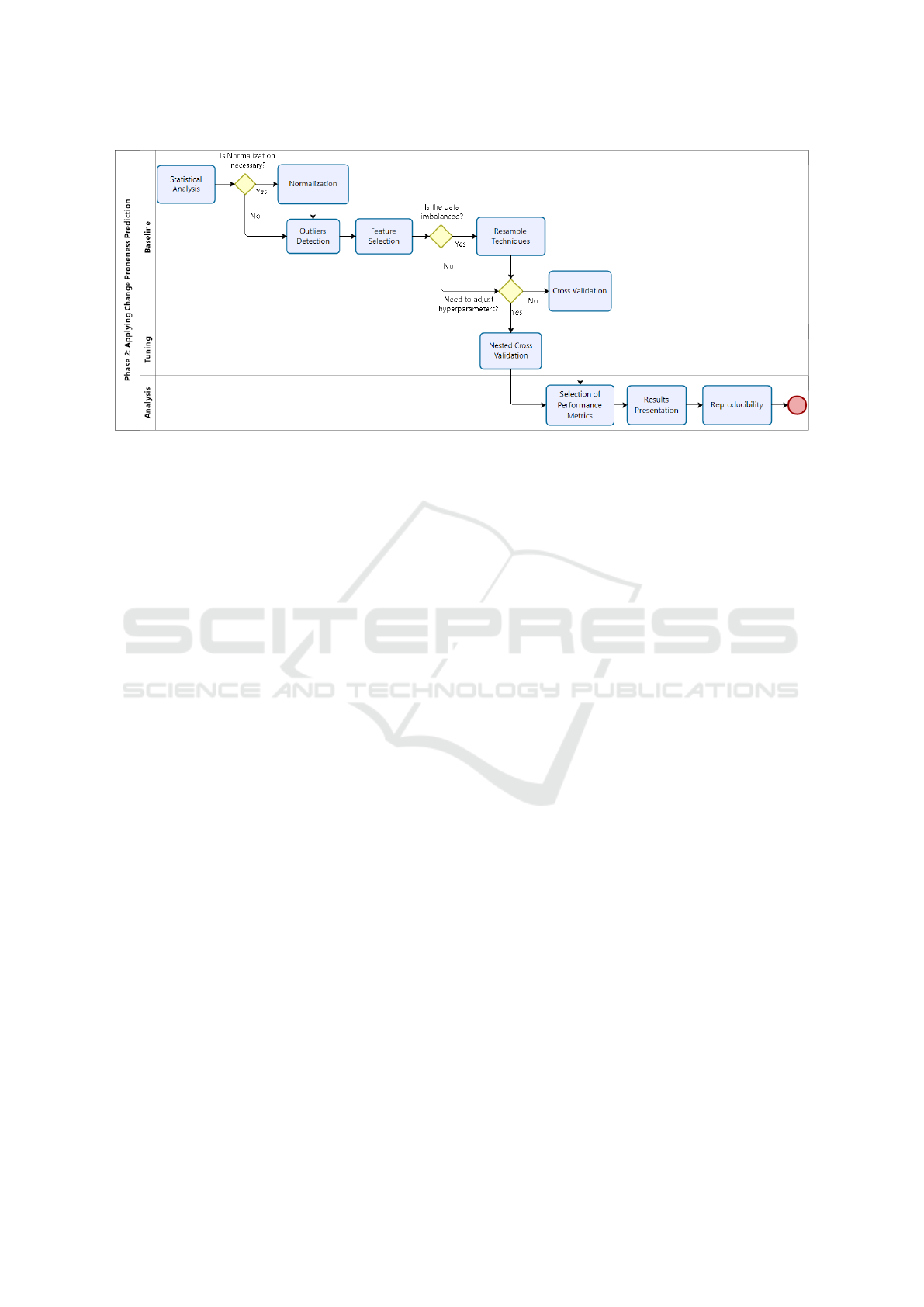
Figure 2: Phase 2 - Applying Change-Proneness Prediction.

Lines of Code (LOC). The domain of change-prone

prediction can be either labels 0-1 to indicate whether

there was some alteration or not.

3.1.3 Collect Metrics

This step consists in collect the metrics chosen previ-

ously (independent and dependent variables) from a

given software project. (Singh et al., 2013) cite a list

of tools to collect the most common metrics accord-

ing to used programming language (JAVA, C++, C#,

etc). At the end of this phase, a proper data set was

built.

3.2 Phase 2: Applying Prediction

The second phase in the proposed guide aims to build

change-prone class prediction models. A prediction

model is designed by learning from historical labeled

data in a supervised way. Besides, this phase encom-

passes the activities related to the analysis of the pre-

diction model performance metrics, the presentation

of the results and the ensure of the experiments re-

producibility. Figure 2 illustrates the activities that

composes the second phase of the proposed guide.

3.2.1 Statistical Analyses

Initially, a general analysis of the data set is strongly

recommended. The software engineer can build a ta-

ble containing, for each feature, a set of important in-

formation, such as: minimum, maximum, mean, me-

dian (med) and standard deviation (SD) values. As-

sess the correlation between the features, e.g. Pearson

Correlation, is high recommended as well. This is re-

lated to the fact that the generated prediction model

may be highly biased by correlated features, then it is

important to identify those correlations.

3.2.2 Normalization

Next, it is essential to check if the features are in

the same scale. For example, two features A and B

may have two different ranges: the ﬁrst one a range

between zero and one, meanwhile the second one a

range in the integers domain. In this case, it is nec-

essary to normalize all features in the data set. There

are different strategies to normalize data. However,

it is important to emphasize that the normalization

approach must be chosen according to the nature of

the investigated problem and the used prediction algo-

rithm. For example, for activation function in neural

network is recommended that the data be normalized

between 0.1 and 0.9 rather than 0 and 1 to avoid sat-

uration of the sigmoid function. Normalization tech-

niques to deal with these scenarios are Min-Max nor-

malizarion or Z-score (Han et al., 2012).

3.2.3 Outlier Detection

Outliers are extreme values that deviate from other

observations on data, i.e., an observation that diverges

from an overall pattern on a sample. Detected outliers

are candidates for aberrant data that may otherwise

adversely lead to model mispeciﬁcation, biased pa-

rameter estimation and incorrect result. It is therefore

important identify them prior to create the prediction

model.

A survey to distinguish between univariate vs.

multivariate techniques and parametrics (Statistical)

vs. nonparametrics procedures has done by (Ben-

Gal, 2005). Detecting outliers is possible only when

multivariate analysis is performed and the interactions

A Practical Guide to Support Change-proneness Prediction

271

among variables are compared with the class of data.

In the other words, an instance can be a multivariate

outlier but a usual data in each feature and an instance

can have values that are outliers in several features but

the whole instance might be a usual multivariate data.

As example, there are two techniques to detect

outliers: Interquartile Range (an univariate paramet-

ric approach) and K-distance of an instance (a multi-

variate nonparametric approach).

3.2.4 Feature Selection

High dimensionality data is problematic for classiﬁ-

cation algorithms due to high computational cost and

memory usage. So, it is important to check if all fea-

tures in the data set are indeed necessary. The main

beneﬁts from feature selection techniques are reduce

the dimensionality space, remove redundant, irrele-

vant or noisy data and performance improvement to

gain in predictive accuracy.

Feature selection methods can be distinguished

into three categories: ﬁlters, wrappers, and embed-

ded/hybrid method. Wrapper methods are brute-force

feature selection which exhaustively evaluates all pos-

sible combinations of the input features, and then ﬁnd

the best subset. Filter methods have low computa-

tional cost but inefﬁcient reliability in classiﬁcation

compared to wrapper methods. Hybrid/ embedded

methods are developed which utilize advantages of

both ﬁlters and wrappers approaches. A hybrid ap-

proach uses both an independent test and performance

evaluation function of the feature subset.

3.2.5 Resample Techniques for Imbalanced Data

Machine Learning techniques require an efﬁcient

training data set, which have an amount similar of in-

stances of the classes; however, in real world prob-

lems some data sets can be imbalanced i.e. a ma-

jority class containing most samples meanwhile the

other class contains few samples, this one generally of

our interest. Using imbalanced data sets to train mod-

els leads to higher misclassiﬁcations for the minority

class. It occurs because there is a lack of information

about the minority class.

The state-of-the-art methods which deal with im-

balanced data for classiﬁcation problems can be cat-

egorized into two main groups: Under-sampling

(US): it refers to the process of reducing the num-

ber of instances of the majority class. Over-sampling

(OS): It consists of generating synthetic data in the

minority class in order to balance the proportion of

data.

For imbalanced multiple classes classiﬁcation

problems, (Fernandez et al., 2013) have done an ex-

perimental analysis to determine the behaviour of the

different approaches proposed in the specialized liter-

ature. (Vluymans et al., 2017) also proposed an ex-

tension to multi-class data using one-vs-one decom-

position.

It is important to mention that is necessary to sepa-

rate the imbalanced data set into two sub sets: training

and test. After that, any of the techniques aforemen-

tioned should only be applied in the training set. The

Figure 3 shows how must to be this splitting approach.

MODEL

CLASSIFIER

RESAMPLE

TECHNIQUES

TEST SET

TRAINING

SET

OUTPUT

ORIGINAL

IMBALANCED

DATA SET

STEP 1 STEP 2 STEP 3

Figure 3: Splitting and Resampling Data Set.

3.2.6 Cross Validation

Training an algorithm and evaluating its statistical

performance on the same data yields an overopti-

mistic result. Cross Validation (CV) was raised to ﬁx

this issue, starting from the remark that testing the

output of the algorithm on new data would yield a

good estimate of its performance. In most real ap-

plications, only a limited amount of data is available,

which leads to the idea of splitting the data: Part of

data (the training sample) is used for training the algo-

rithm, and the remaining data (the validation sample)

are used for evaluating the performance of the algo-

rithm. The validation sample can play the role of new

data. A single data split yields a validation estimate

of the risk, and averaging over several splits yields a

cross-validation estimate. The major interest of CV

lies in the universality of the data splitting heuristics.

A technique widely used to generalize the model

in classiﬁcation problems is k-Fold Cross Validation.

This approach divides the set in k subsets, or folds, of

approximately equal size. One fold is treated as test

set meanwhile the others k − 1 folds work as training

set. This process occurs k times. According to (James

et al., 2013), a suitable k value is k = 5 or k = 10.

ICEIS 2019 - 21st International Conference on Enterprise Information Systems

272

3.2.7 Tuning the Prediction Model

All the steps presented in this paper so far have served

to show good practicals on how to obtain baseline ac-

cording to machine learning algorithm selected. Tun-

ing it consists in ﬁnding the best possible conﬁgura-

tion of this algorithm at hand, where with best conﬁg-

uration we mean the one that is deemed to yield the

best results on the instances that the algorithm will be

eventually faced with. Tuning machine learning algo-

rithms consist of ﬁnding best set of hyperparameters

which yields the best results. Hyperparameters are

tuned by hand at trial-and-error procedure guided by

some rules of thumb, however, there are papers that

analyze a set of hyperparameters for speciﬁcs algo-

rithms in Machine Learning for tuning them, as (Hsu

et al., 2016) which recommend a grid-search on Sup-

port Vector Classiﬁcation algorithm using RBF ker-

nel.

After deﬁning a grid-search in a speciﬁc region, a

nested cross validation must be used to estimate the

generalization error of the underlying model and its

hyperparameter search. Thus it makes sense to take

advantage of this structure and ﬁt the model iteratively

using a pair of nested loops, with the hyperparameters

adjusted to optimise a model selection criterion in the

outer loop (model selection) and the parameters set to

optimise a training criterion in the inner loop (model

ﬁtting/training).

3.2.8 Selection of Performance Metrics

To evaluate a machine learning model for the classiﬁ-

cation problem is necessary to select the appropriate

performance metrics according to two possible sce-

narios: for balanced or imbalanced data set.

In the case of balanced data sets, metrics like ac-

curacy, precision, recall and speciﬁcity can be used

without more concerns. However, in case of im-

balanced data these metrics are not suitable, since

they can lead to dubious results. For example, ac-

curacy metric is not suitable because it tends to give a

high score due a correct prediction of the bigger class

(Akosa, 2017).

It is important to highlight that in case of imbal-

anced data the more suitable metrics are AUC (Area

Under the ROC Curve) and F-score. These perfor-

mance metrics are suitable for imbalanced data be-

cause they takes the minority classes correctly classi-

ﬁed into account, unlike the accuracy.

3.2.9 Ensure the Reproducibility

The last step in this phase consists in ensure the ex-

periments reproducibility, in order to verify the credi-

bility of proposed study. There are some authors who

have proposed basic rules for reproducible computa-

tional research, as (Sandve et al., 2013) which pro-

posed list ten rules.

4 A CASE STUDY

In order to evaluate the guidelines proposed in this

paper, we performed an exploratory case study using

a large data set, extracted from a wide commercial

software, containing the values of 8 static OO met-

rics. Then, different data analysis techniques were

applied over this data set in order to predict change-

prone classes and get insights about this process.

4.1 Phase 1: Designing the Data Set

4.1.1 Independent Variables

The majority of the metrics obtained in the context of

this work were proposed by (Chidamber and Kemerer,

1994), which quantify the structural properties of the

classes in an OO system. In addition to these metrics,

it was obtained Cyclomatic Complexity proposed by

(McCabe, 1976) and Lines of Code.

4.1.2 Dependent Variable

In this work, the change-proneness was adopted as

the dependent variable in order to investigate its rela-

tionship with the independent variables presented in

the previous subsection, following the deﬁnition pro-

posed by (Lu et al., 2012). The authors deﬁne that a

class will be labeled as 1 if in the next release occurs

alteration in the LOC independent variable.

4.1.3 Collect Metrics

The data set of this work is generated from the back-

end source code of a WEB application started in

2013, and until 2018 were collected 8 releases to an-

alyze change-prone classes. This application has in-

volved the development of modules which manages

the needs of multinationals related to processes, such

as return control of merchandise and product quality.

The back-end system has been implemented in C#

totaling 4183 classes; all its features were collected

through the Visual Studio NDepends plugin. At the

end of this phase, a data set containing the values of 8

static OO metrics, for 4183 classes, in 8 releases was

built. Now, it is possible to use this information to

predict change-prone classes.

A Practical Guide to Support Change-proneness Prediction

273

4.2 Phase 2: Applying Prediction

4.2.1 Environment Setup

The exploratory case study presented in this section

was developed using Python 3.7 through the Ana-

conda platform and Jupyter Notebook 5.6.0.

4.2.2 Statistical Analysis

As the ﬁrst step of this phase, we performed a gen-

eral statistic analysis of the proposed data set. Table

1 shows the descriptive statistics of this data set for

each feature.

Table 1: Descriptive Statistics.

Metric Min Max Mean Med SD

LOC 0 1369 36.814 12 91.211

CBO 0 162 7.107 3 12.305

DIT 0 7 0.785 0 1.764

LCOM 0 1 0.179 0 0.289

NOC 0 189 0.612 0 6.545

RFC 0 413 9.966 1 25.694

WMC 0 56 1.558 0 4.244

CC 0 488.0 15.918 8 30.343

4.2.3 Normalization

Since there are features with a different scale the data

set was normalized using min-max normalization into

[0,1] range. For example, LCOM and LOC have dif-

ferent ranges: [0,1] and [0,1369], respectively.

4.2.4 Outlier Detection

The next step was to investigate the existence of out-

liers. In order to do this, we used the box plot method,

for each feature. However, since the proposed data set

contains 8 features, we used a multivariate strategy to

remove outliers, which is described as follows. If an

instance contains at least 4 features with outliers, it

will be dropped. Table 2 shows the number of in-

stances with label 0 and 1, before and after outliers

removal.

Table 2: Overview of the Data Set Before and After Outliers

Removal.

0 1 Total

Before outliers removal 3871 312 4183

After outliers removal 3637 287 3924

4.2.5 Feature Selection

The proposed data set has 8 features. So, not all

features may be necessary or even useful to gener-

ate good predictive models. Therefore, it is neces-

sary to investigate some feature selection methods.

Thus, in this step we explored four (three univariate

and one multivariate) feature selection methods and

compared their results in order to choose the best set

of features. More precisely, we used Chi-square (CS),

One-R (OR), Information Gain (IG) and Symmetrical

Uncertainty (SU). The last one is a multivariate con-

cept in Correlation-based Feature technique.

Table 3 shows the results obtained of each feature

selection techniques for each metric, that is, the rele-

vance of the metric in a speciﬁc method.

Another criteria to determine the number of fea-

tures to keep is to get the value of the highest sum and

establish a threshold of half of its value. 5 features

contain their sum into [28,14], however, according to

Pearson’s correlation CBO and RFC have value 0.89,

i.e., they are strongly correlated. Since RFC has the

sum less than CBO, RFC is dropped. Therefore, the

features selected were CBO, WMC, CC and LCOM.

Table 3: Feature Selection Results.

CS IG OR SU

∑

CBO 8 7 7 6 28

RFC 7 6 6 5 24

WMC 6 5 6 4 21

CC 4 4 5 3 16

LCOM 3 4 4 3 14

LOC 5 3 3 2 13

DIT 2 2 2 2 8

NOC 1 1 1 1 4

4.2.6 Resample Techniques and Cross Validation

Now, we used the data set to run 10 classiﬁcation

algorithms with the default values of Scikit-Learn

ver. 0.20.0 for its hyperparameters, which is known

as baseline. The 10 classiﬁers explored in this step

were: Logistic Regression, LightGBM (Ke et al.,

2017), XGBoost (Chen and Guestrin, 2016), Deci-

sion Tree, Random Forest, KNN, Adaboost, Gradient

Boost, SVM with Linear Kernel and SVM with RBF

kernel. Each classiﬁer was performed in four differ-

ent scenarios: with and without outliers and with and

without feature selection. Methods like XgBoost and

LightGBM have used random state = 42 and KNN

method has set number of neighbour as 5. To vali-

date these results, a k-fold cross validation was used,

ICEIS 2019 - 21st International Conference on Enterprise Information Systems

274

with k = 10 and the scoring function has been set to

“roc auc” instead of accuracy, default of Scikit-Learn.

However, as the proposed data set is imbalanced,

we rerun all the previous experiments using three

undersample and three oversample techniques: Ran-

dom Under-Sampler, Tomek’s Link (Tomek, 1976),

Edited Nearest Neighbours (Wilson, 1972), Random

Over-Sampler, SMOTE (Chawla et al., 2002) and

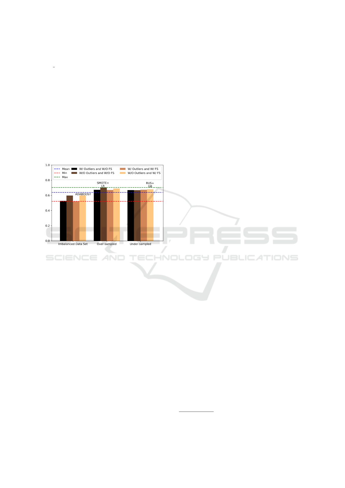
ADASYN (He et al., 2008), respectively. Figure 4

shows the results of these experiments. The x-axis

shows the AUC metric and y-axis the different sce-

narios. The best evaluation founded was using over-

sampled technique: SMOTE + Logistic Regression,

without outliers and without feature selection with

AUC 0.703 and SD ±0.056.

Figure 4: Performance Evaluation in Different Baselines

Scenarios.

4.2.7 Tuning the Prediction Model

This step aims to explore a region of hyperparame-

ters in order to improve the results. The grid search

function was used to performing hyperparameters op-

timization. The nested cross validation, i.e., the outer

cross validation used to generalize the model and the

inner cross validation used to validate the hyperpa-

rameters during the training phase have been set k =

10 for both of them.

In this step, we have used the data set in the most

recommended scenario by this guideline: without out-

liers and keeping only selected features (as deﬁned

in section 4.2.5). We did so because this scenario

presents the data set more reﬁned and possibly more

clear from noisy data. Besides, we have used the same

ten classiﬁers and the same six resample techniques as

in previous section.

We can punctuate that, in general, the AUC ob-

tained by tuning the models outperforms the AUC ob-

tained from baseline experiments. Besides, the best

result from this scenario in this phase outperforms

even the best AUC from any of the scenarios base-

line. This occurs using Random Under Sampler +

SVM Linear got an AUC 0,710. For this result, the

grid search was set as C: [0.002, 1, 512, 1024, 2048]

and Class Weight: [1:1, 1:10, 1:15, 1:20].

However, it is always important to warn that tun-

ing is not a silver bullet. For instance, we performed

the tuning over the model with the best result from

baseline experiments and achieved a worse model

where AUC has decreased from 0.703 to 0.699.

4.2.8 Ensure the Reproducibility

The results of all experiments run in this exploratory

case study are available in a public Github reposi-

tory

. This repository consists of two main folders:

data set and case study. The former contains a csv ﬁle

where all instances used in this paper are into, deﬁned

in section 4.1.

5 CONCLUSIONS

In this paper, we presented a guide to support change-

proneness prediction in order to standardize a mini-

mum list of activities and roadmaps for optimal use

of predictive models in software change-proneness.

For the purpose of validating the proposed guide, we

performed it over a strongly imbalanced data set ex-

tracted from a wide commercial software, contain-

ing 8 static object-oriented metrics proposed by C&K

and McCabe. Additionally, we investigated empirical

studies about change-proneness prediction containing

balanced and imbalanced data sets in order to detect

missing points which our guide considers indispens-

able steps to guarantee minimally good results. As

future works, we plan to apply the proposed guide in

other commercial and open-source data sets. Besides,

we will explore another set of metrics, such as code

smells, design patterns and evolution metrics.

ACKNOWLEDGEMENTS

This research was funded by LSBD/UFC.

REFERENCES

Akosa, J. S. (2017). Predictive accuracy : A misleading

performance measure for highly imbalanced data. In

SAS Global Forum.

https://github.com/cristmelo/PracticalGuide.git

A Practical Guide to Support Change-proneness Prediction

275

Amoui, M., Salehie, M., and Tahvildari, L. (2009). Tempo-

ral software change prediction using neural networks.

International Journal of Software Engineering and

Knowledge Engineering, 19(07):995–1014.

Bansal, A. (2017). Empirical analysis of search based algo-

rithms to identify change prone classes of open source

software. Computer Languages, Systems & Struc-

tures, 47:211–231.

Ben-Gal, I. (2005). Outlier Detection, pages 131–146.

Springer US, Boston, MA.

Catolino, G., Palomba, F., Lucia, A. D., Ferrucci, F., and

Zaidman, A. (2018). Enhancing change prediction

models using developer-related factors. Journal of

Systems and Software, 143:14 – 28.

Chawla, N. V., Bowyer, K. W., Hall, L. O., and Kegelmeyer,

W. P. (2002). Smote: Synthetic minority over-

sampling technique. Journal of Artiﬁcial Intelligence

Research, 16:321–357.

Chen, T. and Guestrin, C. (2016). Xgboost: A scalable tree

boosting system. CoRR, abs/1603.02754.

Chidamber, S. and Kemerer, C. (1994). A metrics suite for

object oriented design. IEEE Transaction on Software

Engineering, 20(6).

Elish, M., Aljamaan, H., and Ahmad, I. (2015). Three em-

pirical studies on predicting software maintainability

using ensemble methods. Soft Computing, 19.

Elish, M. O. and Al-Rahman Al-Khiaty, M. (2013). A

suite of metrics for quantifying historical changes to

predict future change-prone classes in object-oriented

software. Journal of Software: Evolution and Process,

25(5):407–437.

Fernandez, A., Lpez, V., Galar, M., del Jesus, M. J., and

Herrera, F. (2013). Analysing the classiﬁcation of im-

balanced data-sets with multiple classes: Binarization

techniques and ad-hoc approaches. Knowledge-Based

Systems, 42:97 – 110.

Han, J., Kamber, M., and Pei, J. (2012). Data Mining: Con-

cepts and Techniques. Morgan Kaufman, 3rd edition

edition.

He, H., Bai, Y., Garcia, E. A., and Li, S. (2008). Adasyn:

Adaptive synthetic sampling approach for imbalanced

learning. In 2008 IEEE International Joint Confer-

ence on Neural Networks (IEEE World Congress on

Computational Intelligence), pages 1322–1328.

Hsu, C.-W., Chang, C.-C., and Lin, C.-J. (2016). A practical

guide to support vector classiﬁcation.

James, G., Witten, D., Hastie, T., and Tibshirani, R. (2013).

An Introduction to Statistical Learning with Applica-

tions in R. Springer.

Kaur, A., Kaur, K., and Jain, S. (2016). Predicting software

change-proneness with code smells and class imbal-

ance learning. In 2016 International Conference on

Advances in Computing, Communications and Infor-

matics (ICACCI), pages 746–754.

Ke, G., Meng, Q., Finley, T., Wang, T., Chen, W., Ma, W.,

Ye, Q., and Liu, T.-Y. (2017). Lightgbm: A highly

efﬁcient gradient boosting decision tree. In Advances

in Neural Information Processing Systems 30, pages

3146–3154. Curran Associates, Inc.

Khomh, F., Penta, M. D., and Gueheneuc, Y. (2009). An

exploratory study of the impact of code smells on soft-

ware change-proneness. In 2009 16th Working Con-

ference on Reverse Engineering, pages 75–84.

Koru, A. G. and Liu, H. (2007). Identifying and charac-

terizing change-prone classes in two large-scale open-

source products. Journal of Systems and Software,

80(1):63 – 73.

Lu, H., Zhou, Y., Xu, B., Leung, H., and Chen, L.

(2012). The ability of object-oriented metrics to pre-

dict change-proneness: a meta-analysis. Empirical

Software Engineering, 17(3).

Malhotra, R. and Khanna, M. (2014). Examining the effec-

tiveness of machine learning algorithms for prediction

of change prone classes. In 2014 International Con-

ference on High Performance Computing Simulation

(HPCS), pages 635–642.

McCabe, T. J. (1976). A complexity measure. IEEE Trans-

action on Software Engineering.

Posnett, D., Bird, C., and D

evanbu, P. (2011). An em-

pirical study on the inﬂuence of pattern roles on

change-proneness. Empirical Software Engineering,

16(3):396–423.

Runeson, P. and H

ost, M. (2009). Guidelines for conduct-

ing and reporting case study research in software engi-

neering. Empirical software engineering, 14(2):131–

164.

Sandve, G. K., Nekrutenko, A., Taylor, J., and Hovig,

E. (2013). Ten simple rules for reproducible com-

putational research. PLOS Computational Biology,

9(10):1–4.

Singh, P., Singh, S., and Kaur, J. (2013). Tool for generating

code metrics for c# source code using abstract syntax

tree technique. ACM SIGSOFT Software Engineering

Notes, 38:1–6.

Tomek, I. (1976). Two modiﬁcations of cnn. IEEE Trans.

Systems, Man and Cybernetics, 6:769–772.

van Koten, C. and Gray, A. R. (2006). An application of

bayesian network for predicting object-oriented soft-

ware maintainability. Inf. Softw. Technol., 48(1):59–

67.

Vluymans, S., Fern

andez, A., Saeys, Y., Cornelis, C., and

Herrera, F. (2017). Dynamic afﬁnity-based classiﬁca-

tion of multi-class imbalanced data with one-versus-

one decomposition: a fuzzy rough set approach.

Knowledge and Information Systems, pages 1–30.

Wilson, D. L. (1972). Asymptotic properties of nearest

neighbor rules using edited data. IEEE Transactions

on Systems, Man, and Cybernetics, SMC-2(3):408–

421.

Zhou, Y., Leung, H., and Xu, B. (2009). Examining the po-

tentially confounding effect of class size on the asso-

ciations between object-oriented metrics and change-

proneness. IEEE Transactions on Software Engineer-

ing, 35(5):607–623.

ICEIS 2019 - 21st International Conference on Enterprise Information Systems

276