A Comparative Analysis of Android Malware

Neeraj Chavan, Fabio Di Troia and Mark Stamp

Department of Computer Science, San Jose State University, San Jose, California, U.S.A.

Keywords:

Malware, Android, Machine Learning, Random Forest, Logistic Model Tree, Artiﬁcial Neural Network.

Abstract:

In this paper, we present a comparative analysis of benign and malicious Android applications, based on static

features. In particular, we focus our attention on the permissions requested by an application. We consider both

binary classiﬁcation of malware versus benign, as well as the multiclass problem, where we classify malware

samples into their respective families. Our experiments are based on substantial malware datasets and we

employ a wide variety of machine learning techniques, including decision trees and random forests, support

vector machines, logistic model trees, AdaBoost, and artiﬁcial neural networks. We ﬁnd that permissions are

a strong feature and that by careful feature engineering, we can signiﬁcantly reduce the number of features

needed for highly accurate detection and classiﬁcation.

1 INTRODUCTION

As of 2017, the Android OS accounted for more

than 85% of the mobile OS market, and there were

more than 82 billion application (app) downloads

from the Google Play store during 2017 (Android Sta-

tistics, 2017). Predictably, the number of Android

malware apps is also large—it is estimated that there

were 3.5 million such apps in 2017, representing more

than a six-fold increase since 2015 (Malware Fore-

cast, 2017). It follows that effective malware de-

tection on Android devices is of critical importance.

Features that can be collected without executing

the code are said to be “static,” while features that re-

quire execution (or emulation) are considered “dyna-

mic.” Dynamic analysis is generally more informative

and dynamic features are typically more difﬁcult for

malware writers to defeat via obfuscation (Damoda-

ran et al., 2017). However, extracting dynamic featu-

res is likely to be far more costly and time consuming,

as compared to most static features. Since efﬁciency

is important on a mobile platform, in this paper, we

focus on static analysis. Speciﬁcally, we consider

the related problems of Android malware detection

and classiﬁcation based on requested permissions—

features that are easily obtained from the manifest

ﬁle. We analyze this feature over substantial mal-

ware datasets, and we consider the problem of fea-

ture reduction in some detail. Perhaps somewhat sur-

prisingly, we ﬁnd that a small subset of these featu-

res sufﬁces. This is signiﬁcant, since malware de-

tection on a mobile device must be fast, efﬁcient, and

effective—the approach consider here meets all three

of these criteria.

The remainder of this paper is organized as fol-

lows. In Section 2, we brieﬂy discuss relevant back-

ground topics, including related work. In Section 3

we discuss our experimental design and give our ex-

perimental results. We also provide some discussion

of our results. Finally, in Section 4 we conclude the

paper and give some suggestions for future work.

2 BACKGROUND

In this section, we ﬁrst brieﬂy discuss relevant back-

ground topics. First, we outline each of the machine

learning techniques considered in this paper. Then we

discuss some examples of relevant related work.

2.1 Machine Learning Techniques

In this research, we employ a wide variety of machine

learning techniques. A detailed discussion of these

techniques is well beyond the scope of this paper—

here, we simply provide a high-level overview.

Random forest can be viewed as a generalization of

the simple concept of a decision tree (Breiman

and Cutler, 2001). While decision trees are in-

deed simple, they tend to grossly overﬁt the trai-

ning data, and hence provide little, if any, actual

664

Chavan, N., Di Troia, F. and Stamp, M.

A Comparative Analysis of Android Malware.

DOI: 10.5220/0007701506640673

In Proceedings of the 5th International Conference on Information Systems Security and Privacy (ICISSP 2019), pages 664-673

ISBN: 978-989-758-359-9

“learning.” A random forest overcomes the weak-

ness of decision trees by the use of bagging (i.e.,

bootstrap aggregation), that is, multiple decision

trees are trained using subsets of the data and fe-

atures. Then, a voting procedure based on these

multiple decision trees is typically used to deter-

mine the random forest classiﬁcation. In each of

our random forest experiments, we use 100 trees.

Random trees are a subclass of random forests,

where the bagging only involves the classiﬁers,

not the data. We would generally expect better re-

sults from a random forest, but random trees will

be more efﬁcient. Our random trees results are

based on a single tree.

J48 is a speciﬁc implementation of the C4.5 algo-

rithm (Quinlan, 2018), which is a popular method

for constructing decision trees. We would gene-

rally expect random trees to outperform decision

trees while, as mentioned above, random forests

should typically outperform random trees. Howe-

ver, decision trees are more efﬁcient than random

trees, which are more efﬁcient than random fore-

sts. Thus, it is worth experimenting with all three

of these tree-based algorithms to determine the

proper tradeoff between efﬁciency and accuracy.

Artiﬁcial Neural Network (ANN) represents a

large class of machine learning techniques that at-

tempt to (loosely) model the behavior of neurons

and trained using backpropagation (Stamp, 2018).

While ANNs are not a new concept, having ﬁrst

been proposed in the 1940s, they have found

renewed interest in recent years as computing

power has become sufﬁcient to effectively deal

with “deep” neural network, i.e., networks that

include many hidden layers. Such deep networks

have pushed machine learning to new heights.

For our ANN experiments, we use two hidden

layers, with 10 neurons per layer, the rectiﬁed

linear unit (ReLU) for the activation functions on

the hidden layers, and a sigmoid function for the

output layer. Training consists of 100 epochs,

with the learning rate set at α = 0.001.

Support Vector Machine (SVM) is a popular and

effective machine learning technique. According

to (Bennett and Campbell, 2000), “SVMs are a

rare example of a methodology where geometric

intuition, elegant mathematics, theoretical gua-

rantees, and practical algorithms meet.” When

training an SVM, we attempt to ﬁnd a separating

hyperplane that maximizes the “margin,” i.e., the

minimum distance between the classes in the trai-

ning set. A particularly nice feature of SVMs is

that we can map the input data to a higher dimen-

sional feature space, where we are much more li-

kely to be able to separate the data. And, thanks

to the so-called “kernel trick,” this mapping en-

tails virtually no computational penalty. All of

our SVM experiments are based on a linear ker-

nel function with ε = 0.001.

Logistic Model Tree (LMT) can be viewed as a hy-

brid of decision trees and logistic regression. That

is, in an LMT, decision trees are constructed,

with logistic regression functions at the leaf no-

des (Landwehr et al., 2005). In our LMT experi-

ments, we use a minimum of 15 instances, where

each node is considered for splitting.

Boosting is a general—and generally fairly

straightforward—approach to building a strong

model from a collection of (weak) models. In

this paper, we employ the well-known adaptive

boosting algorithm, AdaBoost (Stamp, 2017a).

Multinomial na

ıve Bayes is a form of na

ıve Bayes

where the underlying probability is assumed to sa-

tisfy a multinomial distribution. In na

ıve Bayes,

we make a strong independence assumption,

which results in an extremely simply “model” that

often performs surprisingly well in practice.

The static analysis can be done using the Java

Bytecode extracted after disassembling the apk ﬁle.

Also we can extract permissions from the manifest

ﬁle. In this paper, we take advantage of the static

analysis using permissions of applications and use

them for detecting malware and also classify different

malware families. The effectiveness of these techni-

ques is analyzed using multiple machine learning al-

gorithms.

2.2 Selected Related Work

The paper (Feng et al., 2014) discusses a tool the

authors refer to as Appopscopy, which implements a

semantic language-based Android signature detection

strategy. In their research, general signatures are cre-

ated for each malware family. Signature matching is

achieved using inter-component call graphs based on

control ﬂow properties and the results are enhanced

using static taint analysis. The authors report an accu-

racy of 90% on a malware dataset containing 1027

samples, with the accuracy for individual families

ranging from a high of 100% to a low of 38%.

In the research (Fuchs et al., 2009), the authors

analyze a tool called SCanDroid that they have deve-

loped. This tool extracts features based on data ﬂow.

The work in (Abah et al., 2015) relies on k-nearest

neighbor classiﬁcation based on a variety of features,

A Comparative Analysis of Android Malware

665

include incoming and outgoing SMS and calls, de-

vice status, running processes, and more. This work

claims that an accuracy of 93.75% is achieved. In the

research (Aung and Zaw, 2013), the authors propose

a framework and test a variety of machine learning al-

gorithms to analyze features based on Android events

and permissions. Experimental results from a data-

set of some 500 malware samples yield a maximum

accuracy of 91.75% for a random forest model.

In the paper (Afonso et al., 2015), the authors pro-

pose a dynamic analysis technique that is focused on

the frequency of system and API calls. A large num-

ber of machine learning techniques are tested on a

dataset of about 4500 malicious Android apps. The

authors give accuracy results ranging from 74.53%

to 95.96%. Again, a random forest algorithm achieves

the best results.

The research (Enck et al., 2010) discusses a dy-

namic analysis tool, TaintDroid. This sophisticated

system analyzes network trafﬁc to search for ano-

malous behavior—the research is in a similar vein

as (Feng et al., 2014), but with the emphasis on efﬁ-

ciency. Another Android system call analysis techni-

que is considered in (Dimja

sevi

c et al., 2015).

Our work is perhaps most closely related to the

research in (Sugunan et al., 2018) and (Kapratwar

et al., 2017) which, in turn, built on the groundbre-

aking work of (Arp et al., 2014) and (Schmeelk et al.,

2015), as well as that in (Zhou et al., 2012). In (Arp

et al., 2014), for example, an accuracy of 93.9% is at-

tained over a dataset of 5600 malicious Android apps.

The paper (Kapratwar et al., 2017) considers static

and dynamic analysis of Android malware based on

permissions and API calls, respectively. A robustness

analysis is presented, and it is suggested that malware

writers can most likely defeat detectors that rely on

permissions. We provide a more careful analysis in

this paper and ﬁnd that such is not the case.

3 EXPERIMENTS AND RESULTS

In this section, we ﬁrst discuss our datasets and fe-

ature extraction process. Then we turn our attention

to feature engineering, that is, we determine the most

signiﬁcant features for use in our experiments. We

also discuss our experimental design before presen-

ting results from a wide variety experiments.

3.1 Datasets

We use the Android Malware Genome Project (Zhou

and Jiang, 2012) dataset. This data consists mainly

of apk ﬁles obtained from various malware forums

and Android markets—these samples have been wi-

dely used in previous research. Labels are included,

which specify the family to which each sample be-

longs. Thus, the data can be used for both binary clas-

siﬁcation (i.e., malware versus benign) and the multi-

class (i.e., family) classiﬁcation problems.

For our benign dataset, we crawled the PlayDrone

project (PlayDrone, 2018), as found on the Internet

Archive (Internet Archive, 2018). The resulting apk

ﬁles might include malicious samples. Therefore, we

used Androguard (Androguard, 2018) to ﬁlter broken

and potentially malicious apk ﬁles. Table 1 gives the

number of malware and benign samples that we obtai-

ned. These samples will be used in our binary classi-

ﬁcation (malware versus benign) and multiclass (mal-

ware family) experiments discussed below.

Table 1: Datasets.

Samples

Experiment Type Number

Detection

Malware 989

Benign 2657

Classiﬁcation Malware 1260

3.2 Feature Extraction

To extract static features, we need to reverse en-

gineer the apk ﬁles. We again use Androguard

this reverse engineering task. The manifest ﬁle,

AndroidManifest.xml, contains numerous potential

static features; here we focus on the permissions re-

quested by an application.

From the superset of malware and benign samples,

we ﬁnd that there are 230 distinct permissions. Thus,

for each apk, a feature vector is generated based on

these permissions. The feature vector is simply a bi-

nary sequence of length 230, which indicates whether

each of the corresponding permissions is requested by

the application or not. Along with each feature vec-

tor, we have a denoting label of +1 or −1, indicating

whether the sample is malware or benign, respecti-

vely. The overall architecture, in the case of binary

classiﬁcation, is given in Figure 1.

Figure 1: Binary classiﬁcation architecture.

ForSE 2019 - 3rd International Workshop on FORmal methods for Security Engineering

666

For the multiclass (family) classiﬁcation problem,

essentially the same process is followed as for the bi-

nary classiﬁcation case. However, we only examine

malware samples, and over our malware dataset, we

ﬁnd that only 118 distinct permissions occur. Thus,

the feature vectors for the multiclass problem are of

length 118.

3.3 Feature Engineering

It is likely that many of the features under considera-

tion (i.e., permissions) provide little or no discrimina-

ting information, with respect to the malware versus

benign or the malware classiﬁcation problem. It is

useful to remove such features from the analysis, as

they essentially act as noise, and can therefore cause

us to obtain worse results than we would with a smal-

ler, but more informative, feature set. It is also useful

to remove extraneous features so that scoring is as ef-

ﬁcient as possible. Consequently, our immediate goal

is to determine features that are of no value for our

analysis, and remove them from subsequent conside-

ration.

There are several techniques for determining fea-

ture signiﬁcance. Here we consider two distinct ap-

proaches to this problem. First, we use information

gain to reduce the feature set. Second, we use recur-

sive feature elimination (RFE) based on a linear SVM.

Information gain is easily computed and gives us a

straightforward means of eliminating features. RFE

is somewhat more involved, but accounts for feature

interactions in a way that a simple information gain

calculation cannot.

The information gain (IG) provided by a feature

is deﬁned as the expected reduction in entropy when

we branch on that feature. In the context of a decision

tree, information gain can be computed as the entropy

of the parent node minus the average weighted en-

tropy of its child nodes. We measure the information

gain for each feature, and select features in a greedy

manner. In a decision tree, this has the desirable effect

of putting decisions based on the most informative fe-

atures closest to the root. This is desirable, since the

entropy is reduced as rapidly as possible, and enables

the tree to be simpliﬁed by trimming features that pro-

vide little or no gain.

For our purposes, we simply use the information

gain to reduce the number of features, then apply va-

rious machine learning techniques to this reduced fe-

ature set. Based on the information gain, we selected

the 74 highest ranked features—the top 10 of these

features are given in Table 2. Features that ranked

outside the top 74 provided no improvement in our

results.

Table 2: Permissions ranked by IG.

Score Permission

0.30682 READ SMS

0.28129 WRITE SMS

0.17211 READ PHONE STATE

0.15197 RECEIVE BOOT COMPLETED

0.14087 WRITE APN SETTINGS

0.13045 RECEIVE SMS

0.10695 SEND SMS

0.10614 CHANGE WIFI STATE

0.10042 INSTALL PACKAGES

0.10019 RESTART PACKAGES

As mentioned above, we also reduce the feature

set using RFE based on a linear SVM. In a linear

SVM, a weight is assigned to each feature, with the

weight signifying the importance that the SVM atta-

ches to the feature. For our RFE approach, we elimi-

nate the feature with the lowest linear SVM weight,

then train a new SVM on this reduced (by one) fea-

ture set. Then we again eliminate the feature with the

lowest SVM weight, train a new linear SVM on this

reduced feature set. This process is continued until

a single feature remains, and in this way, we obtain

a complete ranking of the features. The potential ad-

vantage of this RFE technique is that it accounts for

feature interactions among all of the reduced feature

sets. The top 10 features obtained using RFE based

on a linear SVM are listed in Table 3.

Table 3: Permissions ranked by RFE using a linear SVM.

Rank Permission

1 WRITE APN SETTINGS

2 WRITE CALENDAR

3 WRITE CALL LOG

4 WRITE CONTACTS

5 WRITE INTERNAL STORAGE

6 WRITE OWNER DATA

7 WRITE SECURE SETTINGS

8 WRITE SETTINGS

9 WRITE SMS

10 WRITE SYNC SETTINGS

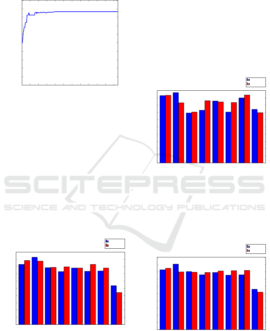
In Figure 2, we give the cross validation score of

the linear SVM as a function of the number of fe-

atures, as obtained by RFE. We see that the top 82

features gives us an optimal result—additional featu-

res beyond this number provide no beneﬁt. Conse-

quently, we use the 82 top RFE features in our expe-

riments below.

A Comparative Analysis of Android Malware

667

20 40

80 100 120 140

160

180 200 220

0.50

0.55

0.60

0.65

0.70

0.75

0.80

0.85

0.90

0.95

1.00

Features

Cross validation score

Figure 2: Recursive feature elimination (RFE).

3.4 Binary Classiﬁcation

In this section, we discuss our binary classiﬁcation

experiments. We consider both the IG features and

the RFE features. We test a wide variety of machine

learning algorithms and provide various statistics.

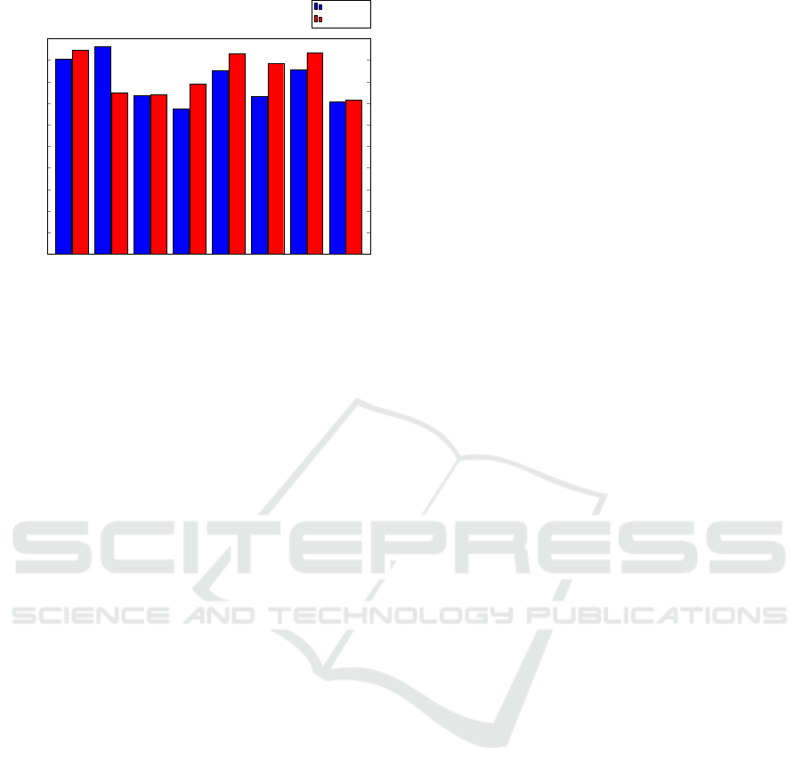
First, we consider the IG features, as discussed in

Section 3.3, above. Bar graphs of training and tes-

ting precision for each of the techniques discussed

in Section 2.1 are plotted in Figure 3. For this ex-

periment the number of samples in the malware and

benign datasets are listed in Table 1, where we see

that there is total of 3647 samples. Here, and in all

subsequent experiments, we use 5-fold cross valida-

tion. Cross validation serves to maximize the num-

ber of test cases, while simultaneously minimizing

the effect of any bias that might exist in the training

data (Stamp, 2017b).

Random forest

ANN

Linear SVM

J48

LMT

Random tree

AdaBoost

Multinomial NB

0.80

0.82

0.84

0.86

0.88

0.90

0.92

0.94

0.96

0.98

1.00

Precision

Training

Testing

Figure 3: Machine learning comparison based on precision

(IG features).

Given a scatterplot of experimental results, an

ROC curve is obtained by graphing the true positive

rate versus the false positive rate, as the threshold va-

ries through the range of values. The area under the

ROC curve (AUC) is between 0 and 1, inclusive, and

can be interpreted as the probability that a randomly

selected positive instance scores higher than a rand-

omly selected negative instance (Stamp, 2017b). In

Figure 4, we give the AUC statistic for the same set

of IG feature experiments that we ahve summarized

in Figure 3.

Random forest

ANN

Linear SVM

J48

LMT

Random tree

AdaBoost

Multinomial NB

0.80

0.82

0.84

0.86

0.88

0.90

0.92

0.94

0.96

0.98

1.00

AUC

Training

Testing

Figure 4: Machine learning comparison based on AUC (IG

features).

We repeated the experiments above using the 82

RFE features, rather than the 74 IG features. The pre-

cision results for these machine learning experiments

are given in Figure 5, while the corresponding AUC

results are summarized in Figure 6.

Random forest

ANN

Linear SVM

J48

LMT

Random tree

AdaBoost

Multinomial NB

0.80

0.82

0.84

0.86

0.88

0.90

0.92

0.94

0.96

0.98

1.00

Precision

Training

Testing

Figure 5: Machine learning comparison based on precision

(RFE features).

ForSE 2019 - 3rd International Workshop on FORmal methods for Security Engineering

668

Random forest

ANN

Linear SVM

J48

LMT

Random tree

AdaBoost

Multinomial NB

0.80

0.82

0.84

0.86

0.88

0.90

0.92

0.94

0.96

0.98

1.00

AUC

Training

Testing

Figure 6: Machine learning comparison based on AUC

(RFE features).

The performance between the various machine

learning algorithms varies signiﬁcantly, with mul-

tinomial na

ıve Bayes consistently the worst, while

random forests and ANNs perform the best. The IG

and RFE cases are fairly similar, although ANNs are

better on the RFE features, with random forest are

better on the IG features.

3.5 ANN Experiments

Since ANNs performed well in the experiments

above, we have conducted additional experiments to

determine the effect of an imbalanced dataset and to

test the effect of small training sets. For these expe-

riments, we use the IG features and the same binary

classiﬁcation dataset as above, with the skewed trai-

ning sets selected at random. Again, we use 5-fold

cross validation.

We experiment with three different ratios between

the sizes of the malware and benign sets, namely, a

ratio of 1:3 (i.e., three times as many benign samples

as malware samples), as well as ratios of 1:6 and 1:12.

For the 1:3 ratio, we have sufﬁcient data to consider

following four different cases:

• 100 malware and 300 benign

• 200 malware and 600 benign

• 400 malware and 1200 benign

• 800 malware and 2400 benign

For a 1:6 ratio, we have enough samples so that we

can consider the following three cases:

• 100 malware and 600 benign

• 200 malware and 1200 benign

• 400 malware and 2400 benign

Finally, for the 1:12 ratio, we have sufﬁcient data for

the following two cases:

• 100 malware and 1200 benign

• 200 malware and 2400 benign

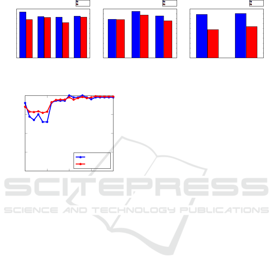
The testing precision and AUC results for the 1:3,

1:6, and 1:12 training cases are given in Figures 7 (a)

through (c), respectively. We see that, for example,

with only 100 malware and 300 benign samples, we

obtain a testing precision in excess of 0.98 and an

AUC of approximately 0.96. Overall, these results

show that the ANN performs extremely well, even

with a small and highly skewed training set. This is

signiﬁcant, since we would like to train a model as

soon as possible (in which case the training set may

be small), and the samples are likely to be highly ske-

wed towards the benign case.

3.6 Robustness Experiments

As an attack on permissions-based detection, a mal-

ware writer might simply request more of the permis-

sions that are typical of benign samples, while still

requesting permissions that are necessary for the mal-

ware to function. In this way, the permissions statis-

tics of the malware samples would be somewhat clo-

ser to those of the benign samples. Analogous attacks

have proven successful against malware detection ba-

sed on opcode sequences (Lin and Stamp, 2011).

To simulate such an attack, for each value of N =

0, 1, 2, . . . , 20, we include the top N benign permissi-

ons in each malware sample. For each of these cases,

we have performed an ANN experiment, similar to

those in Section 3.5, above. The precision and AUC

results are given in the form of line graphs in Figure 8.

Note that the N = 0 case corresponds to no modiﬁca-

tion to the malware permissions.

The results in Figure 8 show that there is a de-

crease in the effectiveness of the ANN when a small

number of the most popular benign permissions are

requested. However, when more than N = 5 permis-

sions are included, the success of the ANN recovers,

and actually improves on the unmodiﬁed N = 0 case.

These results show that a straightforward attack on the

permissions can have a modest effect, but we also see

that permissions are a surprisingly robust feature.

3.7 Multiclass Classiﬁcation

For the multiclass experiments in this section, we

again use permission-based features. The metrics

considered here are precision and the AUC. As above,

we use ﬁve-fold cross validation in each experiment.

For these experiments, we use all malware sam-

ples in our dataset that include a family label. The

distribution of these malware families is given in

A Comparative Analysis of Android Malware

669

100:300

200:600

400:1200

800:2400

0.80

0.82

0.84

0.86

0.88

0.90

0.92

0.94

0.96

0.98

1.00

Precision

AUC

100:600

200:1200

400:2400

0.80

0.82

0.84

0.86

0.88

0.90

0.92

0.94

0.96

0.98

1.00

Precision

AUC

100:1200

200:2400

0.80

0.82

0.84

0.86

0.88

0.90

0.92

0.94

0.96

0.98

1.00

Precision

AUC

(a) Ratio of 1:3 (a) Ratio of 1:6 (a) Ratio of 1:12

Figure 7: ANN results for various malware to benign ratios.

0.80

0.85

0.90

0.95

1.00

Precision

AUC

Figure 8: Robustness tests based on ANN.

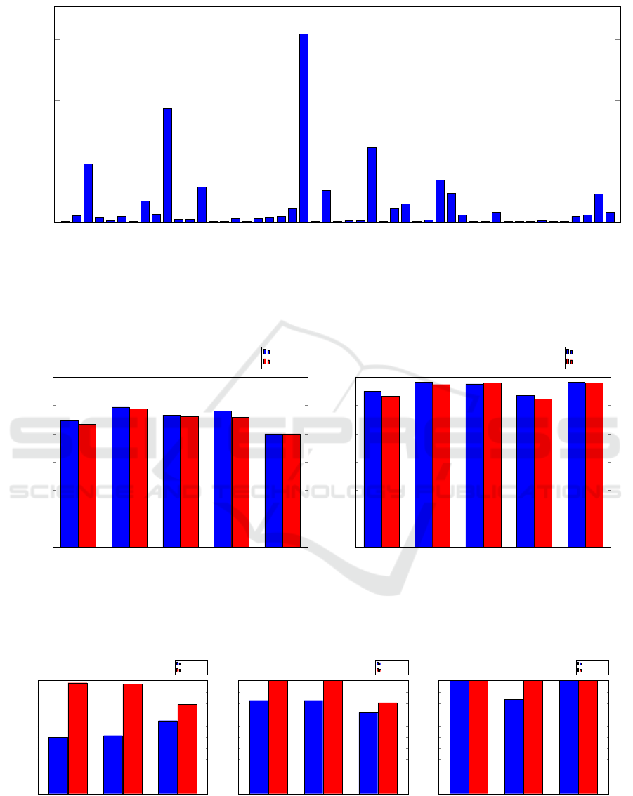
Figure 9. Note that we have 49 malware families and

a total 1260 malware samples.

Bar graphs of precision and AUC results for mul-

tiple machine learning techniques are give in Figu-

res 10 (a) and (b), respectively. We observe that a

random forest performs best in these multiclass expe-

riments, attaining a testing accuracy in excess of 0.95.

This is an impressive number, given that we have such

a large number of classes. Other machine learning

techniques that perform well on this challenging mul-

ticlass problem include LMT and AdaBoost.

While there are 49 malware families in our data-

set, from Figure 9 we see that a few large families do-

minate, while many of the “families” contain only 1

or 2 samples, and most are in the single digits. To

determine the effect of this imbalance on our results,

we also performed multiclass experiments on balan-

ced datasets. In Figures 11 (a) through (c) we give

results for balanced sets with 30, 40, and 50 samples

per family, respectively. For example, 11 of the 49

malware families in our dataset have at least 30 sam-

ples. From each of these 11 families, we randomly

select 30 samples, then perform multiclass experi-

ments and we give the precision and AUC results in

Figure 11 (a).

Overall the results in Figure 11 clearly demon-

strate that our strong multiclass results are not an ar-

tifact of the imbalance in our dataset. In fact, with a

sufﬁcient number of samples per family, we obtain

better results on the balanced dataset than on the

highly imbalanced dataset. Of course, the number of

families is much smaller in the balanced case, but we

do have a signiﬁcant number of families in all of these

experiments.

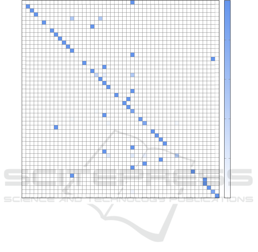
Since a random forest performs best in the mal-

ware classiﬁcation problem, we give the confusion

matrices for this case in Figure 12. This confusion

matrix provides a more ﬁne-grained view of the re-

sults reported above. We observe that the misclassiﬁ-

cation are sporadic, in the sense that all of cases where

a signiﬁcant percentage of samples are misclassiﬁed

occur in small families, with the number of samples

being in the single digits.

4 CONCLUSION

The work in (Kapratwar et al., 2017) considered both

permissions (i.e., a static feature) and system calls

(i.e., a dynamic feature), and the interplay between

the two. The authors concluded that a slight reduction

in the number of permissions has a signiﬁcant effect,

and suggested that malware writers may be able to

evade detection by relatively minor modiﬁcations to

their code, such as reducing the number of permis-

sions requested. Here, we provided a more nuan-

ced analysis to show that it is likely to be signiﬁ-

cantly more difﬁcult to evade permission-based de-

tection than suggested in (Kapratwar et al., 2017).

Speciﬁcally, in this paper we showed that a relatively

small number of permissions can serve as a strong

feature vector, even for the more challenging multi-

class problem. These results indicate that eliminating

the speciﬁc permissions that comprise the reduced fe-

ature set is likely not an option for most malware.

In addition, we showed that taking the opposite tack,

ForSE 2019 - 3rd International Workshop on FORmal methods for Security Engineering

670

FakeNetﬂix

SndApps

DroidKungFu4

BeanBot

RogueLemon

Gone60

SMSReplicator

DroidKungFu1

Zsone

AnserverBot

HippoSMS

GingerMaster

Pjapps

Walkinwat

DogWars

GPSSMSSpy

GGTracker

FakePlayer

Asroot

Bgserv

ADRD

DroidKungFu3

DroidKungFuUpdate

KMin

Spitmo

Tapsnake

CruseWin

BaseBridge

Endofday

YZHC

DroidKungFu2

Jifake

DroidKungFuSapp

Geinimi

GoldDream

zHash

DroidDeluxe

LoveTrap

DroidDream

GamblerSMS

Zitmo

NickyBot

NickySpy

CoinPirate

DroidCoupon

RogueSPPush

Plankton

DroidDreamLight

jSMSHider

100

200

300

187

309

122

Number of samples

Figure 9: Distribution of malware families.

J48

Random forest

LMT

Linear SVM

AdaBoost

0.70

0.75

0.80

0.85

0.90

0.95

1.00

Precision

Training

Testing

J48

Random forest

LMT

Linear SVM

AdaBoost

0.70

0.75

0.80

0.85

0.90

0.95

1.00

AUC

Training

Testing

(a) Precision (b) AUC

Figure 10: Multiclass results.

Random forest

LMT

Linear SVM

0.80

0.82

0.84

0.86

0.88

0.90

0.92

0.94

0.96

0.98

1.00

Precision

AUC

Random forest

LMT

Linear SVM

0.80

0.82

0.84

0.86

0.88

0.90

0.92

0.94

0.96

0.98

1.00

Precision

AUC

Random forest

LMT

Linear SVM

0.80

0.82

0.84

0.86

0.88

0.90

0.92

0.94

0.96

0.98

1.00

Precision

AUC

(a) 30 samples (11 families) (b) 40 samples (9 families) (c) 50 samples (7 families)

Figure 11: Multiclass results with balanced datasets (testing).

A Comparative Analysis of Android Malware

671

FakeNetﬂix

SndApps

DroidKungFu4

BeanBot

RogueLemon

Gone60

SMSReplicator

DroidKungFu1

Zsone

AnserverBot

HippoSMS

GingerMaster

Pjapps

Walkinwat

DogWars

GPSSMSSpy

GGTracker

FakePlayer

Asroot

Bgserv

ADRD

DroidKungFu3

DroidKungFuUpdate

KMin

Spitmo

Tapsnake

CruseWin

BaseBridge

Endofday

YZHC

DroidKungFu2

Jifake

DroidKungFuSapp

Geinimi

GoldDream

zHash

DroidDeluxe

LoveTrap

DroidDream

GamblerSMS

Zitmo

NickyBot

NickySpy

CoinPirate

DroidCoupon

RogueSPPush

Plankton

DroidDreamLight

jSMSHider

FakeNetﬂix

SndApps

DroidKungFu4

BeanBot

RogueLemon

Gone60

SMSReplicator

DroidKungFu1

Zsone

AnserverBot

HippoSMS

GingerMaster

Pjapps

Walkinwat

DogWars

GPSSMSSpy

GGTracker

FakePlayer

Asroot

Bgserv

ADRD

DroidKungFu3

DroidKungFuUpdate

KMin

Spitmo

Tapsnake

CruseWin

BaseBridge

Endofday

YZHC

DroidKungFu2

Jifake

DroidKungFuSapp

Geinimi

GoldDream

zHash

DroidDeluxe

LoveTrap

DroidDream

GamblerSMS

Zitmo

NickyBot

NickySpy

CoinPirate

DroidCoupon

RogueSPPush

Plankton

DroidDreamLight

jSMSHider

100

50 50

100

38 13 50

100

1 1 1

2 1

2 2

100

19 19

13 50

100

2 2 2

100

Figure 12: Random forest confusion matrix as percentages (training).

that is, adding unnecessary permissions that are com-

mon among bening apps, is also of limited value. We

conclude that features based on permissions are likely

to remain a viable option for detecting Android mal-

ware.

Our experimental results also show that malware

detection on an Android device is practical, since the

necessary features can be extracted and scored efﬁ-

ciently. For example, using an ANN on a reduced

feature set, we can obtain an AUC of 0.9920 for the

binary classiﬁcation problem. And even in the case of

highly skewed data—as would typically be expected

in a realistic scenario—an ANN can attain a testing

accuracy in excess of 96%.

The malware classiﬁcation problem is inherently

more challenging than the malware detection pro-

blem. But even in this difﬁcult case, we obtained a

testing accuracy of almost 95%, based on a random

forest. It is worth noting that a random forest also per-

forms well for binary classiﬁcation, with about 97%

testing accuracy. A random forest requires signiﬁ-

cantly less computing power to train, as compared

to an ANN, and this might be a factor in some im-

plementations, although training is often considered

one-time work.

For future work, it would be interesting to further

explore deep learning for Android malware detection,

based on permissions. For ANNs, there are many pa-

rameters that can be tested, and it is possible that the

ANN results presented in this paper can be signiﬁ-

cantly improved upon. As another avenue for future

work, recent research has shown promising malware

detection results by applying image analysis techni-

ques to binary executable ﬁles; see, for example (Hu-

ang et al., 2018; Yajamanam et al., 2018). As far as

the authors are aware, such analysis has not been app-

lied to the mobile malware detection or classiﬁcation

problems.

ForSE 2019 - 3rd International Workshop on FORmal methods for Security Engineering

672

REFERENCES

Abah, J., V, W. O., B, A. M., M, A. U., and S,

A. O. (2015). A machine learning approach

to anomaly-based detection on Android platforms.

https://arxiv.org/abs/1512.04122.

Afonso, V. M., de Amorim, M. F., Gr

egio, A. R. A., Jun-

quera, G. B., and de Geus, P. L. (2015). Identi-

fying Android malware using dynamically obtained

features. Journal of Computer Virology and Hacking

Techniques, 11(1):9–17.

Androguard (2018). Androguard: Github repository. https:

//github.com/androguard/androguard.

Android Statistics (2017). Android statistics marketers

need to know. http://mediakix.com/2017/08/android-

statistics-facts-mobile-usage/.

Arp, D., Spreitzenbarth, M., Hubner, M., Gascon, H., and

Rieck, K. (2014). DREBIN: effective and explai-

nable detection of android malware in your pocket.

In Proceedings of the 2014 Network and Distribu-

ted System Security Symposium, NDSS 2014. The In-

ternet Society. http://wp.internetsociety.org/ndss/wp-

content/uploads/sites/25/2017/09/11 3 1.pdf.

Aung, Z. and Zaw, W. (2013). Permission-based Android

malware detection. International Journal of Scientiﬁc

& Technology Research, 2(3).

Bennett, K. P. and Campbell, C. (2000). Support vector ma-

chines: Hype or hallelujah? SIGKDD Explorations,

2(2):1–13.

Breiman, L. and Cutler, A. (2001). Random

forests

. https://www.stat.berkeley.edu/

∼

breiman/

RandomForests/cc home.htm.

Damodaran, A., Troia, F. D., Visaggio, C. A., Austin, T. H.,

and Stamp, M. (2017). A comparison of static, dyna-

mic, and hybrid analysis for malware detection. Jour-

nal of Computer Virology and Hacking Techniques,

13(1):1–12.

Dimja

sevi

c, M., Atzeni, S., Ugrina, I., and Rakamari

Z. (2015). Evaluation of android malware de-

tection based on system calls. Technical Report

UUCS-15-003, School of Computing, University of

Utah. http://www.cs.utah.edu/docs/techreports/2015/

pdf/UUCS-15-003.pdf.

Enck, W., Gilbert, P., Chun, B.-G., Cox, L. P., Jung, J., Mc-

Daniel, P., and Sheth, A. N. (2010). TaintDroid: An

information-ﬂow tracking system for realtime privacy

monitoring on smartphones. In Proceedings of the

9th USENIX Conference on Operating Systems De-

sign and Implementation, OSDI’10, pages 393–407.

USENIX Association.

Feng, Y., Anand, S., Dillig, I., and Aiken, A. (2014).

Apposcopy: Semantics-based detection of Android

malware through static analysis. In Proceedings of

the 22nd ACM SIGSOFT International Symposium on

Foundations of Software Engineering, pages 576–587.

Fuchs, A. P., Chaudhuri, A., and Foster, J. S. (2009).

SCanDroid: Automated security certiﬁcation of An-

droid applications. https://www.cs.umd.edu/

∼

avik/

papers/scandroidascaa.pdf.

Huang, W., Troia, F. D., and Stamp, M. (2018). Robust

hashing for image-based malware classiﬁcation. In

ICETE (1), pages 617–625. SciTePress.

Internet Archive (2018). Internet Archive. https://archive.

org.

Kapratwar, A., Troia, F. D., and Stamp, M. (2017).

Static and dynamic analysis of android malware.

In Proceedings of the 1st International Works-

hop on Formal Methods for Security Engineering,

ForSE 2017, in conjunction with the 3rd Interna-

tional Conference on Information Systems Security

and Privacy (ICISSP 2017), pages 653–662. Sci-

TePress. http://www.scitepress.org/DigitalLibrary/

PublicationsDetail.aspx?ID=mI9FBvhgap4=&t=1.

Landwehr, N., Hall, M., and Frank, E. (2005). Logistic

model trees. Machine Learning, 59(1-2):161–205.

Lin, D. and Stamp, M. (2011). Hunting for undetectable

metamorphic viruses. Journal in Computer Virology,

7(3):201–214.

Malware Forecast (2017). Malware forecast:

The onward march of Android malware.

https://nakedsecurity.sophos.com/2017/11/07/2018-

malware-forecast-the-onward-march-of-android-

malware/.

PlayDrone (2018). PlayDrone: A me-

asurement study of Google Play.

https://systems.cs.columbia.edu/projects/playdrone/.

Quinlan, R. (2018). Software available for download. http:

//www.rulequest.com/Personal/.

Schmeelk, S., Yang, J., and Aho, A. (2015). Android mal-

ware static analysis techniques. In Proceedings of the

10th Annual Cyber and Information Security Research

Conference, CISR ’15, pages 5:1–5:8, New York, NY,

USA. ACM.

Stamp, M. (2017a). Boost your knowledge of adaboost.

https://www.cs.sjsu.edu/

∼

stamp/ML/ﬁles/ada.pdf.

Stamp, M. (2017b). Introduction to Machine Learning with

Applications in Information Security. Chapman and

Hall/CRC, Boca Raton.

Stamp, M. (2018). Deep thoughs on deep learning. https:

//www.cs.sjsu.edu/

∼

stamp/ML/ﬁles/ann.pdf.

Sugunan, K., Gireesh Kumar, T., and Dhanya, K. A. (2018).

Static and dynamic analysis for android malware de-

tection. In Rajsingh, E. B., Veerasamy, J., Alavi,

A. H., and Peter, J. D., editors, Advances in Big Data

and Cloud Computing, pages 147–155, Singapore.

Springer Singapore.

Yajamanam, S., Selvin, V. R. S., Troia, F. D., and Stamp,

M. (2018). Deep learning versus gist descriptors for

image-based malware classiﬁcation. In ICISSP, pages

553–561. SciTePress.

Zhou, Y. and Jiang, X. (2012). Dissecting android mal-

ware: Characterization and evolution. In Proceedings

of the 2012 IEEE Symposium on Security and Privacy,

SP ’12, pages 95–109, Washington, DC, USA. IEEE

Computer Society.

Zhou, Y., Wang, Z., Zhou, W., and Jiang, X. (2012). Hey,

you, get off of my market: Detecting malicious apps in

ofﬁcial and alternative Android markets. In 19th An-

nual Network and Distributed System Security Sympo-

sium, NDSS 2012.

A Comparative Analysis of Android Malware

673