Using Recurrent Neural Networks for Action and Intention Recognition

of Car Drivers

Martin Torstensson

, Boris Duran

and Cristofer Englund

2,3

Chalmers University of Technology, Gothenburg, Sweden

RISE Viktoria, Lindholmspiren 3A, SE 417 56 Gothenburg, Sweden

Center for Applied Intelligent Systems Research (CAISR), Halmstad University, SE 301 18 Halmstad, Sweden

Keywords:

CNN, RNN, Optical Flow.

Abstract:

Trafﬁc situations leading up to accidents have been shown to be greatly affected by human errors. To reduce

these errors, warning systems such as Driver Alert Control, Collision Warning and Lane Departure Warning

have been introduced. However, there is still room for improvement, both regarding the timing of when a

warning should be given as well as the time needed to detect a hazardous situation in advance. Two factors that

affect when a warning should be given are the environment and the actions of the driver. This study proposes

an artiﬁcial neural network-based approach consisting of a convolutional neural network and a recurrent neural

network with long short-term memory to detect and predict different actions of a driver inside a vehicle. The

network achieved an accuracy of 84% while predicting the actions of the driver in the next frame, and an

accuracy of 58% 20 frames ahead with a sampling rate of approximately 30 frames per second.

1 INTRODUCTION

Trafﬁc safety is today one of the major global soci-

etal challenges and trafﬁc accidents has become one

of the most common causes of death among young

persons (World Health Organization (WHO), 2015).

Human errors are one of the major factors affecting

the situations leading up to trafﬁc accidents (Singh,

2015). Among the systems used today to reduce hu-

man errors are warning systems. Examples of these

warning systems are Driver Alert Control, Collision

Warning and Lane Departure Warning

. The inten-

tion of such systems is either to alert the driver of a

hazardous situation or about a certain condition. This

study explores ways to further improve such systems

by taking into account the future state of the driver.

1.1 Related Work

Recurrent neural networks (RNN) with long short-

term memories (LSTM) have previously been used by

(Jain et al., 2016), (Olabiyi et al., 2017) for driver ac-

tion prediction, to predict for example breaking and

lane changes. Methods based on sensor fusion were

https://volvo.custhelp.com/app/manuals/

ownersmanualinfo/year/2018/model/V60

applied to data from e.g. the CAN bus, GPS and cam-

eras. The camera input did, in both cases, contain

at least one camera directed at the driver’s face. In

(Jain et al., 2016) a precision of 90.5% and a recall of

87.4% was achieved with 3.16 seconds-to-maneuver.

The focus of these studies are maneuvers and even

though images of the driver were used to predict these

maneuvers they did not cover the state of the driver.

Another method used for prediction of lane

changes was presented in (Pech et al., 2014). The

main concept of the study was to use eye gaze of the

driver for predictions ten seconds in advance. The in-

formation was, in turn, extracted from the angle and

position of the driver’s head. An overall accuracy of

75% was reached. This type of methodology provides

a way to make predictions a long time in advance

however it is sensitive to the position of the drivers

head and what windows the driver looks through and

what mirrors the driver use. In the case of actions

inside the vehicle, the drivers focus on windows and

mirrors might not provide the same information as the

driver might be looking at the road while trying to

reach something inside of the car.

Other studies have focused on the behavior of the

driver, such as (Carmona et al., 2015) a study of the

driver’s level of aggressiveness in different environ-

ments. The inputs used were mainly based on the

232

Torstensson, M., Duran, B. and Englund, C.

Using Recurrent Neural Networks for Action and Intention Recognition of Car Drivers.

DOI: 10.5220/0007682502320242

In Proceedings of the 8th International Conference on Pattern Recognition Applications and Methods (ICPRAM 2019), pages 232-242

ISBN: 978-989-758-351-3

CAN-bus, an inertial measurement unit and GPS. One

upside to the method used was that it did not require

expensive equipment. A downside, on the other hand,

was an adaption phase at the start of each processed

sequence, where the performance was lowered due to

a lack of information. The case of long-time predic-

tions of driver behavior was considered in (Wijnands

et al., 2018). Among the behaviors studied was accel-

eration and whether the speed of the car was within

the legal limits. The study used GPS coordinates of

a test car, sampled at an interval of 30 seconds over a

large period of time, in combination with other infor-

mation.

The use of CNNs to classify the posture of a driver

has been tested in (Yan et al., 2015). In the study im-

ages of the full body posture of the driver was used

to classify four different classes: drive normal, re-

sponding to a cell phone, eating & smoking and oper-

ating the shift gear. With this method, the authors got

an accuracy of 99.78% correct classiﬁcations on their

dataset. The same dataset was used in (Yan et al.,

2016) however instead divided into six classes: Call,

Eat, Break, Wheel, Phone play, and Smoke. The clas-

siﬁcations were made using a RCNN and achieved a

mean average precision rate of 97.76%.

Optical ﬂow ﬁelds were used in our study as in

order to improve the accuracy of the CNN. This type

of method was also used in (Simonyan and Zisser-

man, 2014). In that study, both the original images

and the optical ﬂow ﬁelds were processed in parallel

and the intermediate results were concatenated at the

end of the network. The study’s results were better or

close to the compared methods containing among oth-

ers improved dense trajectories and Spatio-temporal

HMAX. The results suggested that the use of opti-

cal ﬂow gave a better performance compared to raw

frames.

To the best of our knowledge there are no previous

studies investigating predictions of a driver’s actions

inside a car with the use of neural networks. Under-

standing the driver’s intent and thus the future state of

the driver provides a possibility to further anticipate

the driver’s readiness to react to new conditions in a

trafﬁc situation. Hence, valuable information about

how well a driver could handle a driving task or react

to changes in the environment can be gained. There-

fore warning systems could potentially make use of

such information to provide earlier and more accurate

warnings.

In (Jain et al., 2016) the method used to process

facial images was based on a landmark representation

of the face. It might be possible to generalize this

method, from landmarks of facial images to images

of the whole-body posture. Hence, more information

about the driver could potentially be used as the full

body posture can provide more information.

The architecture proposed in the presented study

revolved around two types of neural networks, one

used for classiﬁcation of images and the other to pre-

dict future events based on sequences of outputs from

the ﬁrst network. A CNN was used for image clas-

siﬁcations, while an RNN with LSTM generated the

action intention recognition. The training and test-

ing images for the networks depicted the whole-body

posture of the driver.

2 DATA

There are currently few public datasets containing

image sequences of drivers. One of the datasets

was created in (Abouelnaga et al., 2017). The fo-

cus of this dataset was distracted drivers and con-

tains the classes: Drive Safe, Talk Passenger, Text

Right, Drink, Talk left, Text Left, talk Right, Adjust

Radio, Hair & Makeup and Reach Behind. Unfortu-

nately, this dataset is not on a sequential form where

one class leads to another creating a chain of actions

and could therefore not be used in this study. An-

other dataset created by (Jain et al., 2015) consists

of 1180 miles of driver data which is annotated with

turns, lane changes and drive straight. This dataset,

even though it contains images of a driver, does not

focus on driver activity. Therefore the dataset was not

suitable for this study.

The dataset used in this study consists of se-

quences of images, collected using two cameras

mounted inside of a car. During data collection, one

camera was placed in the left A-pillar facing the driver

and the other camera on the side window of the front

passenger seat. Due to safety reasons, the car was

parked during the collection of the data. There were

eight participants performing 13 tasks in a Volvo V40

Cross Country. In total eight classes of driver behav-

ior were used: drive safe, glance, lean, remove a hand

from the steering wheel, reach, grab, retract and hold

object. Examples of these classes can be found in Fig-

ure 1. The drivers were instructed to perform tasks in

a speciﬁc order, for example, start by driving safely

then glance, remove a hand from the steering wheel,

lean towards the center then proceed by picking up

an object. Each task was performed ﬁve times by

each participant and lasted between 1.5 and 13 sec-

onds. Around 90,000 images were collected. Due to

technical difﬁculties, the images were captured at ap-

proximately 30 frames per second. The dataset was

then divided into two separate sets where the training

and testing set consisted of 55 and 10 sequences re-

Using Recurrent Neural Networks for Action and Intention Recognition of Car Drivers

233

spectively for each participant. The sequences used

as the test set corresponded to tasks where the driver

was given very few instructions of how the task was

to be performed more than that they would start by

drive safe and then pick up and bring an object to

them. This was to encourage a more natural approach

to how the task was performed. The distributions of

the classes in the training and testing set can be found

in Table 1 for the CNN and in Table 2 for the RNN

with LSTM. A restriction of working with sequences

of actions is that different actions vary in the time it

takes to perform them as well as how often they oc-

cur. It is therefore problematic to create an evenly

distributed dataset. The difﬁculty in using normaliza-

tion in order to even out the dataset is that all different

types of actions can not be expected to be performed

over an equal amount of time or frequency. An exam-

ple is the classes glance and reach, a person might not

need to glance before picking up an object but do need

to reach for it. The test data was also meant to be as

representative as possible of how the actions would be

performed in reality, which also affects the distribu-

tion in the test set. One example is the very low num-

ber of occurrences of lean in the test dataset, which

suggests that the assumption that lean would be an

important class when a driver is picking up an object

might not be true. It could also mean that the objects

were to close to the driver for lean as a class to play a

signiﬁcant role. The RNN with LSTM was tested for

each set of 20 frames in each sequence and evaluated

on the corresponding next 20 frames unless the next

20 frames would reach outside of the sequence.

The CNN used in this study requires one ground

truth class label for each image. In practice, it would

be possible for more than one of the classes to be a

valid label for some of the images. In order to use

only one class as a label for the images, a priority

system was created. The system used the last action

taken by the driver that corresponded to a class as the

label. The exceptions to this rule were the classes

grab, retract and holding object that also had a pri-

ority over the other classes.

3 METHOD

3.1 Model Overview

The system proposed in this study is based on two ma-

jor parts, a CNN for image classiﬁcation and an RNN

with LSTM for action prediction. The CNN and RNN

with LSTM models used in this study were based on

the work by (Torstensson, 2018). A schematic illus-

tration of the system is shown in Figure 2, where the

input to the system is a sequence of images. The

ﬁrst step in the processing chain is to decrease the

size of the images to 256 by 128 pixels and trans-

form them to grayscale in order to reduce the com-

putational cost. After preprocessing, the images are

classiﬁed by the CNN. The classiﬁcation transformed

the two-dimensional image into a scalar representing

the resulting class for the given frame. The prepro-

cessed images are also converted into optical ﬂow

ﬁelds, which are sent into the CNN in parallel to the

original images. The RNN with LSTM then uses the

generated sequence of classes as input to generate a

sequence of scalars representing a prediction of fu-

ture classes. The training process of the CNN and

RNN with LSTM requires a ground truth that can map

each of the images to a speciﬁc class. For benchmark-

ing, two different inputs were given to the RNN, the

ground truth of the actual behavior, and the predicted

output from the CNN. Both the CNN and the RNN

with LSTM used cross-entropy as the objective func-

tion.

3.2 Classiﬁcation

Among the models presented in this study is a plain

CNN model used for classiﬁcation, which consists of

two CNN blocks shown in Figure 3. The dataset was

captured with two cameras, therefore each time frame

provides two images. These images can be separately

classiﬁed, but that can potentially lead to an increase

in errors as well as not making use of the added in-

formation provided by using cameras with different

angles. To make use of this data, two of the CNN

blocks are used in parallel. The outputs are concate-

nated and followed by dense layers. As mentioned in

(Yamashita et al., 2018) dropout layers can be used to

reduce overﬁttning and have therefore been used af-

ter the dense layers. The plain CNN model does not

receive any beneﬁt from using a sequence of images

compared to separate frames. Another model using

dense optical ﬂow as an additional input was created

to make use of the information in the changes be-

tween the images in the sequence. Optical ﬂow can

be used as a method of representing the changes be-

tween images as a vector ﬁeld. This can be done by

imposing two assumptions. These assumptions are

that the pixel values are preserved from one image

to the other, though they might be moved around and

the second one that nearby pixel values are moved at a

similar rate (Fleet and Weiss, 2006). The arrays used

as input to the convolution block was on the form

[Batch size, Image height, Image width, Channels]

where Channels was one when the grayscale images

were sent in and two for the dense optical ﬂow ﬁelds.

ICPRAM 2019 - 8th International Conference on Pattern Recognition Applications and Methods

234

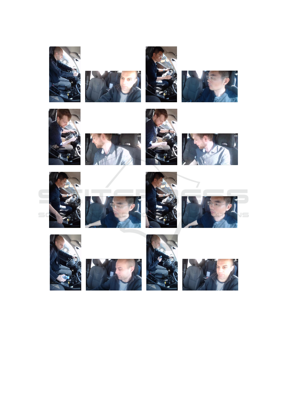
(a) Drive safe (b) Drive safe (c) Glance (d) Glance

(e) Lean (f) Lean (g) Remove hand (h) Remove hand

(i) Reach (j) Reach (k) Grab (l) Grab

(m) Retract (n) Retract (o) Hold (p) Hold

Figure 1: Sample images from the dataset.

The same CNN block can therefore, be used to pro-

cess the optical ﬂow ﬁelds as the CNN block process-

ing the images and does so in parallel but with sepa-

rate weights. The optical ﬂow model can be found in

Figure 4.

3.3 Prediction

One of the differences between a RNN and a CNN

is that the RNN keeps a memory when processing a

sequence. The elements of the network, h

, can be

calculated, given the input x

, at a time t as described

Using Recurrent Neural Networks for Action and Intention Recognition of Car Drivers

235

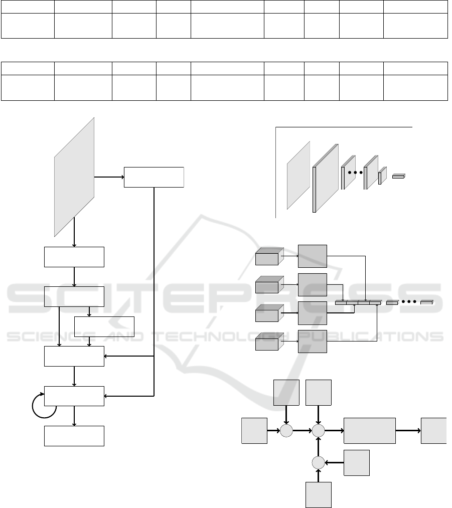
Table 1: Class distributions in testing and training set for the CNN.

Class: Drive safe Glance Lean Remove hand Reach Grab Retract Hold object

Training: 30521 10487 4106 6492 12915 935 3228 7316.

Testing: 6035 578 28 524 2915 268 768 1884

Table 2: Class distributions in testing and training set for the RNN.

Class: Drive safe Glance Lean Remove hand Reach Grab Retract Hold object

Training: 30681 10482 4191 6493 13036 940 3233 7136

Testing: 5944 577 28 522 2915 268 766 1875

Image

Downsample

Ground truth

Grayscale

Optical ﬂow

CNN

LSTM

Output

Figure 2: An illustration of the system used in this study.

in Figure 5. Where W , H are the weights and b a bias

(Jain et al., 2016).

The elements are therefore calculated by also us-

ing the previous elements, this is why it can be viewed

as having a memory as previous inputs also affect the

later ones. One problem with RNNs is known as the

vanishing and exploding gradients problem (Pascanu

et al., 2012).

One way to handle this issue is to use a version of

RNN called RNN with LSTM, which is illustrated in

Figure 6. The intention of adding the LSTM is, in-

stead of storing the information in the hidden unit, to

CNN block

Image

Convolution

Maxpool

Convolution

Maxpool

Figure 3: The structure of the CNN block.

Frontal camera

CNN block

Frontal ﬂow

CNN block

Side camera

CNN block

Side ﬂow

CNN block

DenseDense

Figure 4: The structure of the CNN with optical ﬂow.

Non-linear function

t−1

Figure 5: A chart of an RNN.

use a memory cell for information storage. The mem-

ory cell, c

, is then passed on for each element of the

sequence. The update of the hidden unit is in this case

based on three gates: The input gate (i

), the forget

gate ( f

) and the output gate (o

). These gates deter-

mine the ﬂow of information in and out of the memory

cell as well as the update of the hidden state. The σ is

ICPRAM 2019 - 8th International Conference on Pattern Recognition Applications and Methods

236

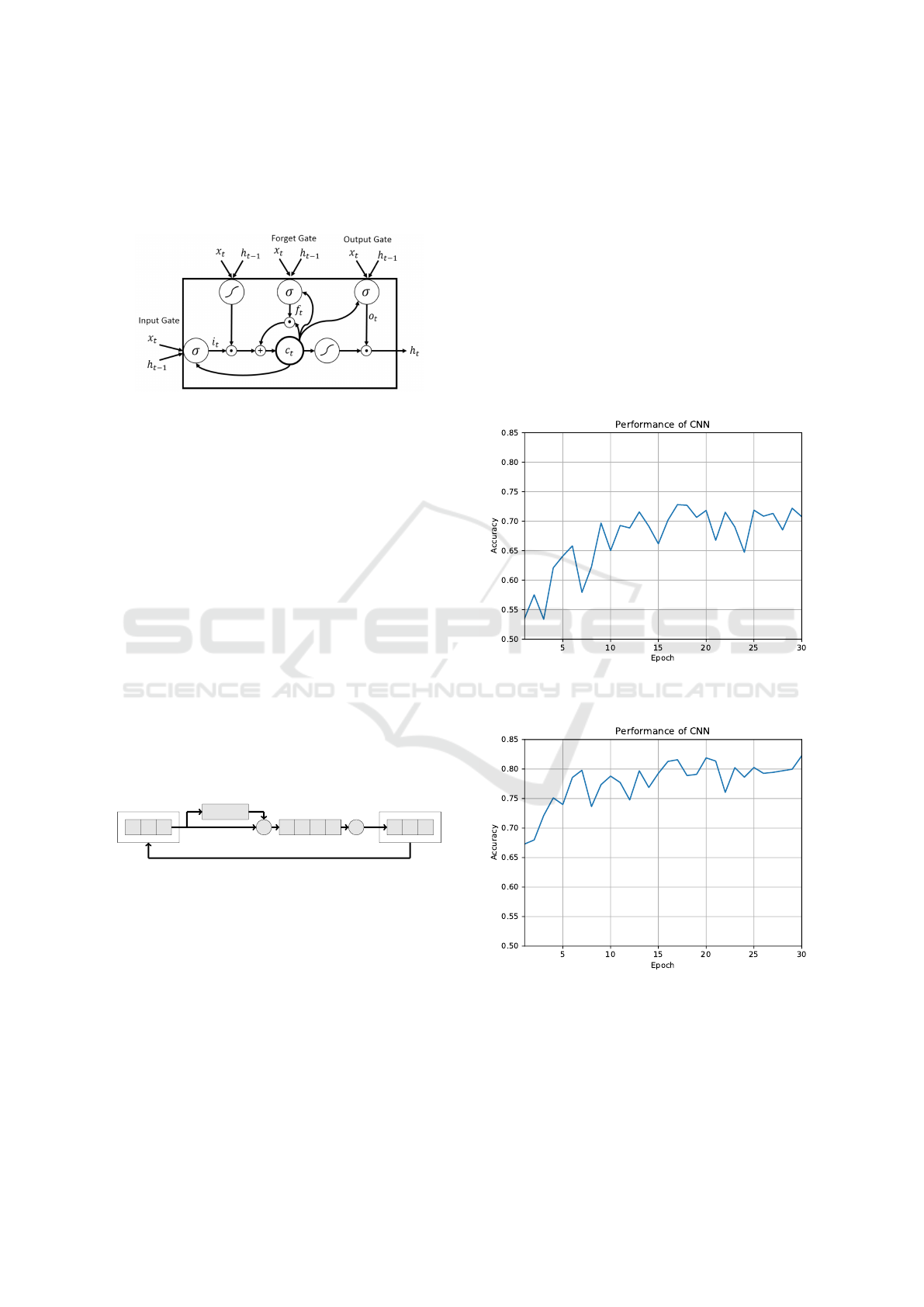
a logistic function, the wave is a non-linearity and x

the input at time t. The beneﬁt of using LSTM is that

the structure uses summations, which reduces the risk

of vanishing or exploding gradients (Jain et al., 2016).

Figure 6: LSTM cell diagram from (Jain et al., 2016).

The main task of the RNN with LSTM presented

in the study is to predict the next element of the in-

put sequence. More speciﬁcally a bidirectional RNN

with LSTM has been used but will be referred to as

RNN with LSTM for simplicity (Schuster and Pali-

wal, 1997). The sequences used as input is either from

the CNN or the ground truth depending on which

model is being used. With a sequence of size t the

predicted element can be added at t = 0 and the last

element is removed. The newly created sequence can

then be used as an input to the RNN with LSTM

to generate yet another element. By repeating this

process, predictions of an inﬁnite number of frames

ahead can be made. The process is illustrated in Fig-

ure 7. When one of the predictions is used as an input

in the following iterations there is a risk that an incor-

rect prediction will lower the accuracy of coming pre-

dictions as the input is incorrect. Using this approach

introduces a risk of propagating errors leading to a

lowered average accuracy for each frame predicted.

t−2

t−1

RNN

t−2

t−1

t+1

t−1

t+1

−

Figure 7: An overview of the prediction process of the RNN

with LSTM proposed in this study.

4 RESULTS

The CNN and RNN with LSTM were trained and

tested separately. The CNN was tested for different

number of epochs, while the RNN was tested for dif-

ferent number of epochs and values of the hyperpa-

rameters. One epoch of training with the CNN us-

ing opticalﬂow took approximately 10 minutes on a

GeForce GTX 1080 Ti. The RNN wih LSTM took

slightly above one minute on the same device.

4.1 Classiﬁcation

Two tests were done on the CNN, one on the plain

CNN, see Section 3.2, and one on the optical ﬂow

CNN. In Figure 8 the results of the plain CNN can be

seen. In this ﬁgure, the x-axis is the number of epochs

trained and the y-axis the accuracy, where the accu-

racy is deﬁned as the number of correctly classiﬁed

images divided by the total number of images. Fig-

ure 9 shows the results of the optical ﬂow CNN. With

the ﬁrst model, the best accuracy achieved was 73%

while the best with the second model was 82%. The

later model performed better and was the one used in

later tests with the RNN.

Figure 8: The accuracy of the CNN for different number of

epochs trained.

Figure 9: The accuracy of the CNN, with the addition of

parallel optical ﬂow input, for different number of epochs

trained.

4.2 Prediction

In order to set the model hyperparameters of the RNN

with LSTM, Bayesian optimization was used. The

Using Recurrent Neural Networks for Action and Intention Recognition of Car Drivers

237

network was ﬁrst tested with random values within

set bounds of the hyperparameters. The hyperparam-

eters, to be tuned this way, were the number of hidden

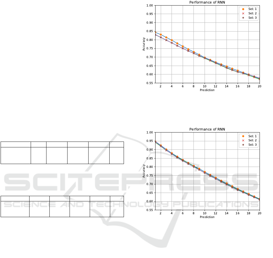
units and layers, and the learning rate. In Figure 10

the results of different sets of hyperparameters can be

found, the input data was from the CNN. The y-axis

is the accuracy and the x-axis the number of frames

predicted into the future. Similarly, the results when

using the ground truth as input the performance for

different sets of hyperparameters can be found in Fig-

ure 11. Testing the RNN with LSTM on the ground

truth data represents a test where the CNN would per-

form perfectly. The best performing hyperparameters,

as well as the search space set for the case of CNN in-

put data and ground truth input data, can be found in

Table 3 and 4 respectively.

Table 3: Hyperparameters used in the test of the RNN with

LSTM on the CNN input data. From left to right are the hy-

perparameter sets shown in Figure 10, best received value,

minimum bound and maximum bound.

Parameter Set:1 Set:2 Set:3 Min Max

Hidden units 50 148 120 50 150

Layers 2 1 2 1 2

Learningrate 0.02 0.00865 0.01610 0.00001 0.02

Table 4: Hyperparameters used in the test of the RNN with

LSTM on the ground truth input data. From left to right are

the hyperparameter sets shown in Figure 11, best received

value, minimum bound and maximum bound.

Parameter Set:1 Set:2 Set:3 Min Max

Hidden units 149 50 50 50 150

Layers 1 2 2 1 2

Learningrate 0.01987 0.01423 0.01555 0.00001 0.02

The RNN with LSTM was tested both on the out-

put from the CNN and the ground truth. Results

from the tests can be found in Figures 12 and 13 re-

spectively. The x-axis represents the number of time

frames predicted into the future and the y-axis the ac-

curacy. The accuracy is deﬁned as the number of cor-

rect predictions divided by the total number of pre-

dictions separately for each of the time steps. The

different lines are varying amounts of epochs trained

and the dotted line a comparison. The intention of

the comparison is to show the case if the predictions

would be a repetition of the last element in the input

as if there would be no transition between classes.

The best results with the CNN input data was 84%

accuracy when predicting one frame ahead and 58%

accuracy when predicting 20 frames ahead. The net-

work outperformed the comparison for all future time

steps with a growing margin for longer time predic-

tions. In the case when using the ground truth data

as input, the best performance gave an accuracy of

96% after one frame and 61% after 20 frames. The

Figure 10: Accuracy of the RNN with LSTM, tested on the

CNN input data, at different numbers of frames predicted.

Each line represents one set of hyperparameters, which can

be founds in Table 3.

Figure 11: Accuracy of the RNN with LSTM, tested on

the ground truth input data, at different numbers of frames

predicted. Each line represents one set of hyperparameters,

which can be found in Table 4.

comparison performed better for very short time pre-

dictions but fell of quicker resulting in a better perfor-

mance of the network with longer time predictions.

There is a clear trend in both cases of dropping accu-

racy with longer time predictions. This could prob-

ably, at least in part, be related to the accumulating

error in the model used.

To further evaluate the performance of the RNN

with LSTM, trained and tested with ground truth data

as input, confusion matrices were created containing

the recall and precision as deﬁned in (Powers, 2008).

The results for one frame predictions can be seen in

Tables 5 and 6, while the 20 frames predictions can

be found in Tables 7 and 8.

Out of all classes, the ones that the model per-

formed best for were drive safe, reach and hold. These

classes were also the ones appearing the most in the

ICPRAM 2019 - 8th International Conference on Pattern Recognition Applications and Methods

238

Table 5: Recall of one frames prediction.

Ground truth

Drive safe Glance Lean Remove hand Reach Grab Retract Hold

Predicted

Drive safe 1.0 0.07 0.04 0.09 0.0 0.0 0.0 0.0

Glance 0.0 0.92 0.04 0.06 0.0 0.0 0.0 0.0

Lean 0.0 0.0 0.79 0.0 0.0 0.0 0.0 0.0

Remove hand 0.0 0.01 0.07 0.84 0.02 0.0 0.0 0.0

Reach 0.0 0.0 0.07 0.0 0.97 0.27 0.0 0.0

Grab 0.0 0.0 0.0 0.0 0.0 0.27 0.0 0.0

Retract 0.0 0.0 0.0 0.0 0.0 0.42 0.81 0.03

Hold 0.0 0.0 0.0 0.0 0.0 0.03 0.19 0.97

Table 6: Precision of one frames prediction.

Ground truth

Drive safe Glance Lean Remove hand Reach Grab Retract Hold

Predicted

Drive safe 0.98 0.01 0.0 0.01 0.0 0.0 0.0 0.0

Glance 0.02 0.92 0.0 0.05 0.01 0.0 0.0 0.0

Lean 0.0 0.0 0.88 0.08 0.0 0.04 0.0 0.0

Remove hand 0.0 0.01 0.0 0.83 0.14 0.0 0.0 0.0

Reach 0.0 0.0 0.0 0.0 0.98 0.02 0.0 0.0

Grab 0.0 0.0 0.0 0.0 0.0 1.0 0.0 0.0

Retract 0.0 0.0 0.0 0.0 0.0 0.16 0.8 0.04

Hold 0.0 0.0 0.0 0.0 0.0 0.01 0.14 0.85

dataset, while the ones appearing signiﬁcantly less

could obtain a value as low as 0%.

5 DISCUSSION

One possible reason for why the CNN could be im-

proved with optical ﬂow is that it works in the time

dimension as well. Hence, information in the se-

quence which is hard to extract from single frames,

such as the direction of movement, can be used. This

effect could also potentially be useful with the priority

system used for annotating the data. One still frame

might not be sufﬁcient to extract the information of

which action was performed last.

The results of the best performing hyperparam-

eters for the RNNs with LSTM showed that differ-

ent sets of hyperparameters performed similarly. It

appeared that the best choice of the number of lay-

ers was one for the ground truth input and two for

the CNN input. The best value of the learning rate

was also high, which might have been due to the low

amount of epochs used in each training phase.

The results in (Jain et al., 2016) and (Pech et al.,

2014) are difﬁcult to compare with the results in this

study due to the differences in timescale and actual

task. The predictions focused on movements of the

car rather than the actions of the driver. Consequently

the timescale differs from the one in this study where

the classes changes constantly during a sequence and

a single class can last a few frames. The sensor fusion

approach used in (Jain et al., 2016) could provide an

interesting prospect of further work if combined with

the method in the study presented here.

The studies (Yan et al., 2015) and (Yan et al.,

2016) achieved higher classiﬁcation accuracy on their

dataset than the one presented here. A major dif-

ference between these studies and the one presented

here is that our study classiﬁes sequences of images

with shifting classes, which the other studies, to our

knowledge, does not. Therefore there are transitions

between the classes, which can be challenging for a

machine or human to classify and therefore contribut-

ing to the difference in classiﬁcation accuracy.

The variation in performance, on different classes,

shown by the confusion matrices could be due to how

the more well-represented classes become more likely

to be predicted as they have a larger probability of ap-

pearing. With an increasing amount of the smaller

classes becoming part of the larger classes in each

iteration the probability of prediction might increase

for the larger classes as they appear more often. This

type of effect could potentially be mitigated with the

use of a bias correction that evens out the probability

of each class being chosen. This type of correction,

on the other hand, run the risk of creating a network

Using Recurrent Neural Networks for Action and Intention Recognition of Car Drivers

239

Table 7: Recall of 20 frames prediction.

Ground truth

Drive safe Glance Lean Remove hand Reach Grab Retract Hold

Predicted

Drive safe 0.94 0.77 0.54 0.79 0.28 0.0 0.0 0.0

Glance 0.05 0.19 0.46 0.08 0.09 0.0 0.0 0.0

Lean 0.0 0.0 0.0 0.0 0.01 0.0 0.0 0.0

Remove hand 0.01 0.03 0.0 0.13 0.12 0.04 0.02 0.0

Reach 0.01 0.0 0.0 0.0 0.51 0.96 0.9 0.23

Grab 0.0 0.0 0.0 0.0 0.0 0.0 0.0 0.0

Retract 0.0 0.0 0.0 0.0 0.0 0.0 0.0 0.01

Hold 0.0 0.0 0.0 0.0 0.01 0.0 0.08 0.76

Table 8: Precision of 20 frames prediction.

Ground truth

Drive safe Glance Lean Remove hand Reach Grab Retract Hold

Predicted

Drive safe 0.65 0.09 0.0 0.07 0.18 0.0 0.0 0.0

Glance 0.29 0.18 0.02 0.06 0.45 0.0 0.0 0.0

Lean 0.0 0.0 0.0 0.0 0.95 0.0 0.0 0.05

Remove hand 0.04 0.04 0.0 0.11 0.74 0.02 0.04 0.01

Reach 0.01 0.0 0.0 0.0 0.51 0.09 0.24 0.15

Grab nan nan nan nan nan nan nan nan

Retract 0.0 0.0 0.0 0.0 0.0 0.0 0.0 1.0

Hold 0.0 0.0 0.0 0.0 0.01 0.0 0.04 0.95

that repeatedly predicts small classes that barely ever

appear and therefore lowers the accuracy. The preci-

sion and recall could potentially also be improved by

using a cost function which uses those measurements.

By changing the cost function there is potential to re-

ward the correct classiﬁcation of the smaller classes

and better adjust to the distribution of the dataset.

It would also be possible to change the dataset

from the system of priority into a system where sev-

eral classes can be used as a label for an image. One

potential beneﬁt of this could be an increase in the ac-

curacy of the CNN with less reliance on the optical

ﬂow. Hierarchical clustering is a method that poten-

tially could be used. If done in a divisive manner one

general class could be split up into subclasses, which

in turn also can be split up into further subclasses. In

such a manner a tree structure of classes could be cre-

ated (Zhang et al., 2017).

The CNN used for classiﬁcation could potentially

be improved by implementing features from some of

the networks performing well in benchmarks such as

ImageNet, one example is GoogleNet (Russakovsky

et al., 2015). The network used could also easily be

replaced with another network trained for the same

type of data as the CNN was used as a separate mod-

ule.

6 CONCLUSIONS

This work presents an RNN with LSTM to predict ac-

tion and intention for car drivers. The proposed sys-

tem consists of two modules: one CNN and one RNN

with LSTM. The CNN classiﬁes images into one of

the eight known action classes. The CNN use four

parallel images as input, two with images from two

different cameras mounted inside the cabin of the test

car and two images that correspond to the optical ﬂow

ﬁelds of the two camera images.

The classiﬁcation accuracy of the CNN was 73%

while using only the two camera images and when

adding the two optical ﬂow images 82% accuracy was

achieved. The RNN with LSTM was used to pre-

dict future intentions of the car driver. The RNN with

LSTM takes as input an array of classiﬁcations made

by the CNN to predict the action in the next frame.

Two approaches were compared. One where the RNN

with LSTM classiﬁcations from the CNN were used

as input and one where the ground truth was used as

input.

The best prediction accuracies achieved was 84%

for one frame ahead predictions and 58% after 20

frames ahead in the case of using the output of the

CNN as input data. When using the ground truth as

input the accuracies were increased to 96% after one

ICPRAM 2019 - 8th International Conference on Pattern Recognition Applications and Methods

240

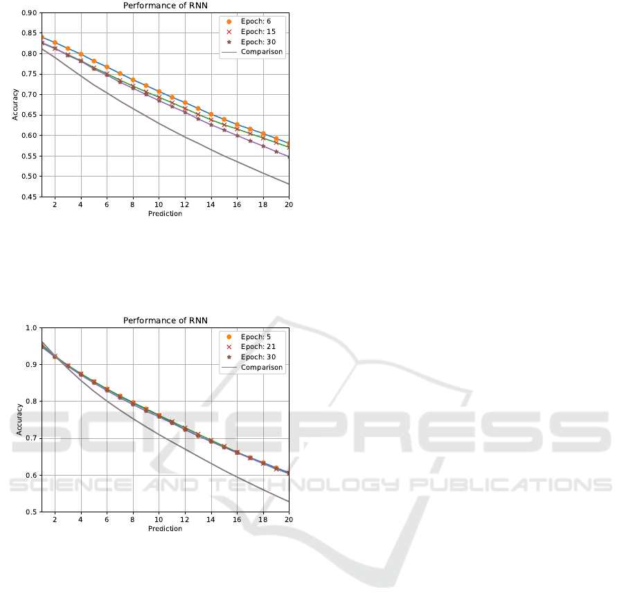
Figure 12: Accuracy of the RNN with LSTM with the best

performing hyperparameters, tested on the CNN input data,

at different numbers of frames predicted. Each line repre-

sents a different amount of epochs trained and the dotted

line is a comparison.

Figure 13: Accuracy of the RNN with LSTM with the best

performing hyperparameters, tested on the ground truth in-

put data, at different numbers of frames predicted. Each

line represents a different amount of epochs trained and the

dotted line is a comparison.

frame ahead and 61% after 20 frames.

ACKNOWLEDGMENT

This work is part of the AIR project (action and

intention recognition in human interaction with au-

tonomous systems), ﬁnanced by the KK foundation

under the grant agreement number 20140220.

REFERENCES

Abouelnaga, Y., Eraqi, H. M., and Moustafa, M. N.

(2017). Real-time distracted driver posture classiﬁ-

cation. CoRR, abs/1706.09498.

Carmona, J., Garca, F., Martn, D., Escalera, A. d. l., and

Armingol, J. M. (2015). Data fusion for driver be-

haviour analysis. Sensors, 15(10):25968–25991.

Fleet, D. and Weiss, Y. (2006). Optical Flow Estimation,

pages 237–257. Springer US, Boston, MA.

Jain, A., Koppula, H. S., Raghavan, B., Soh, S., and Saxena,

A. (2015). Car that knows before you do: Anticipat-

ing maneuvers via learning temporal driving models.

In The IEEE International Conference on Computer

Vision (ICCV).

Jain, A., Singh, A., Koppula, H. S., Soh, S., and Saxena,

A. (2016). Recurrent neural networks for driver ac-

tivity anticipation via sensory-fusion architecture. In

2016 IEEE International Conference on Robotics and

Automation (ICRA), pages 3118–3125.

Olabiyi, O., Martinson, E., Chintalapudi, V., and Guo, R.

(2017). Driver Action Prediction Using Deep (Bidi-

rectional) Recurrent Neural Network. ArXiv e-prints.

Pascanu, R., Mikolov, T., and Bengio, Y. (2012). Un-

derstanding the exploding gradient problem. CoRR,

abs/1211.5063.

Pech, T., Lindner, P., and Wanielik, G. (2014). Head track-

ing based glance area estimation for driver behaviour

modelling during lane change execution. In 17th

International IEEE Conference on Intelligent Trans-

portation Systems (ITSC), pages 655–660.

Powers, D. (2008). Evaluation: From precision, recall and

f-factor to roc, informedness, markedness & correla-

tion. Mach. Learn. Technol., 2.

Russakovsky, O., Deng, J., Su, H., Krause, J., Satheesh,

S., Ma, S., Huang, Z., Karpathy, A., Khosla, A.,

Bernstein, M., Berg, A. C., and Fei-Fei, L. (2015).

ImageNet Large Scale Visual Recognition Challenge.

International Journal of Computer Vision (IJCV),

115(3):211–252.

Schuster, M. and Paliwal, K. K. (1997). Bidirectional re-

current neural networks. IEEE Transactions on Signal

Processing, 45(11):2673–2681.

Simonyan, K. and Zisserman, A. (2014). Two-stream

convolutional networks for action recognition in

videos. In Ghahramani, Z., Welling, M., Cortes, C.,

Lawrence, N. D., and Weinberger, K. Q., editors, Ad-

vances in Neural Information Processing Systems 27,

pages 568–576. Curran Associates, Inc.

Singh, S. (2015). Critical reasons for crashes investigated

in the national motor vehicle crash causation survey.

Washington, DC: National Highway Trafﬁc Safety

Administration. (Trafﬁc Safety Facts CrashStats. Re-

port No. DOT HS 812 115).

Torstensson, M. (2018). Prediction of driver actions with

long short-term memory recurrent neural networks.

Master’s thesis, Chalmers University of Technology.

Retrieved from http://studentarbeten.chalmers.se/.

Wijnands, J. S., Thompson, J., Aschwanden, G. D., and

Stevenson, M. (2018). Identifying behavioural change

Using Recurrent Neural Networks for Action and Intention Recognition of Car Drivers

241

among drivers using long short-term memory recur-

rent neural networks. Transportation Research Part

F: Trafﬁc Psychology and Behaviour, 53:34 – 49.

World Health Organization (WHO) (2015). Global Status

Report on Road Safety 2015. WHO Press, Geneva.

Yamashita, R., Nishio, M., Do, R. K. G., and Togashi, K.

(2018). Convolutional neural networks: an overview

and application in radiology. Insights into Imaging,

9(4):611–629.

Yan, C., Zhang, B., and Coenen, F. (2015). Driving pos-

ture recognition by convolutional neural networks. In

2015 11th International Conference on Natural Com-

putation (ICNC), pages 680–685.

Yan, S., Teng, Y., Smith, J. S., and Zhang, B. (2016).

Driver behavior recognition based on deep convolu-

tional neural networks. In 2016 12th International

Conference on Natural Computation, Fuzzy Systems

and Knowledge Discovery (ICNC-FSKD), pages 636–

641.

Zhang, Z., Murtagh, F., Van Poucke, S., Lin, S., and Lan,

P. (2017). Hierarchical cluster analysis in clinical

research with heterogeneous study population: high-

lighting its visualization with r. Annals of transla-

tional medicine, 5(4):75.

ICPRAM 2019 - 8th International Conference on Pattern Recognition Applications and Methods

242