
Optimal Design of Production Systems: Metaoptimization with
Generalized De Novo Programming
Helena Brožová
1
and Milan Vlach
2
1
Czech University of Life Sciences, Faculty of Economics and Management, Department of Systems Engineering,
Kamýcká 129, Prague 6, Czech Republic
2
Charles University, Faculty of Mathematics and Physics, Department of Theoretical Computer Science and
Mathematical Logic, Malostranské náměstí 25, Prague 1, Czech Republic
Keywords: De Novo Programming, Model Conditions, Capacity Constraints, Requirement Constraints, Multi-Objective
Optimization, Optimal Design.
Abstract: Milan Zelený, in a number of papers, proposed and developed specially structured LP model called De Novo
Programming. This approach uses, in an essential way, a transformation of the original problem to continuous
knapsack problem, and it concerns only models with capacity constraints and some implicit assumptions about
the problem data. Here we extend this methodology to cases involving not only capacity constraints but also
requirement and balance constraints. This extension is based on the methodology of Zelený and uses some
principles of the STEM methods. We present an example of an adaptation of De Novo approach for models
with both capacity, requirement and balance constraints.
1 INTRODUCTION
Optimization of systems means finding "best
available" values of some criterion given a defined
input and output of this system. Optimal design of
systems means "best available" setting of proposed
system. Process of system design requires
understanding the content of three system approach
phases – reality, model and metamodel. In the first
phase the inquiring system is used for description and
understanding the real problem. If we do not
understand the reality, we cannot solve its problems
properly. In the second phase, inquiring system for
creating the model of problem solved is important.
The proper selection of the model is important for
obtaining the good results. In the third phases the
inquiring system of abstract process of model
creation, metamodel is studied (Gigch, 1991).
Production system optimization, in business and
marketing, is methodology for decision process,
which leads to the optimal production mix under the
defined criterion (criteria). Very often the
mathematical programming, especially the linear
optimization model is used to find the optimal
solution. As Zelený (1986, 1990a, 1990b)
emphasises, the already formulated model implicitly
contains the optimal solution. Therefore, the decision
is given by the set parameters of the model. The
crucial problem is how to formulate this model
correctly, respectively, how to choose the best input
data? The question of the best design or formulation
of the model can be seen as a metamodeling process.
A model is the first abstraction of the real-world
problem, and then a metamodel can be seen as the
second abstraction, highlighting and optimizing the
properties of the model itself. Metamodeling typically
involves studying the input, output relationships, and
then fitting right models to represent that behaviour.
Metamodeling identifies the underlying modelling
process and provides tools and techniques for model
development that will allow the proper application to
real problems. In this process, Zelený (1990a, 1990b)
suggests De Novo programming for optimal design of
production systems described by the linear
optimization model with the constraints of the “”
type. This approach is used in practical applications
for instance by Babic and Pavic, (1996), Huang,
Tzeng, (2007) and Zhang et al., 2009. Fiala (2011)
describes the future development and possible
applications of various modifications of De Novo
programming.
The main aim of this paper is to generalize the De
Novo approach for finding of optimal design of
Brožová, H. and Vlach, M.
Optimal Design of Production Systems: Metaoptimization with Generalized De Novo Programming.
DOI: 10.5220/0007682404730480
In Proceedings of the 8th International Conference on Operations Research and Enterprise Systems (ICORES 2019), pages 473-480
ISBN: 978-989-758-352-0
Copyright
c
2019 by SCITEPRESS – Science and Technology Publications, Lda. All rights reserved
473

production system so that more types of constraints
are possible, in particular “≥” and “=”.
2 DE NOVO PROGRAMING
To motivate the De Novo approach to optimal design
of production systems, Zelený (1986, 1990a; 1990b,
2005, 2010) starts with considering the standard
linear programming model for allocating given
resources to possible activities in order to achieve a
given economic objective. If only one criterion is
considered and the objective is to maximize it, then
we have the problem
→ s.t.
,0 (1)
where is a real
,
-matrix, is a real -vector,
and is a real -vector.
When multiple criteria are involved, we have to
solve the multiple objective problem
→ s.
t
.
,0
(2)
where is a real
,
-matrix of coefficients of
objective functions.
An important question is what happens to the
optimal solution if the resource allocation changes.
Therefore, since the early days of linear
programming, both practitioners and theorists have
been interested in behaviour of solutions if
coefficients of the problem vary. Such questions have
led to the emergence of
• Sensitivity analysis (investigation of changes in
the individual coefficients which cause an optimal
solution to become non-optimal);
• Parametric programming (investigation of
changes when some of the coefficients are
functions of parameters);
• Robust optimization (investigation of solutions
under uncertainty that is represented as
deterministic variability in the value of the
parameters);
• Inverse optimization (investigation of solutions
with goal objective value when some of the
coefficients are parameters);
• De Novo programming (investigation of budget
allocation to individual resources which results in
optimal system structure) (Zelený, 1990a, 1990b,
2005, 2010).
The De Novo methodology (Zelený, 1990b) allows
for changes in some of the input data, particularly,
with changes in the components
of the right-hand
side vector of model (1) or (2). Clearly, such
changes describe changes in resources allocation;
modify the system design, and, therefore, the set of
feasible solutions, which may change the optimal
solution. In contrast to the sensitivity analysis and
parametric programming, De Novo programming
similarly as Robust or Inverse optimization requires
some additional exogenous data. De Novo
programming requires specification of cost of
resources and level of available budget.
According to Zelený (1990a, 1990b), if denotes
a given -vector of unit cost of resources and
denotes a given available budget, then De Novo
approach gives to the freedom to vary freely in the
region given by
0.
(3)
To indicate that the components of are now real
variables we change the notation and use the letter
instead of . Now it should be clear that instead
considering the general linear programming problem
(1), (2) resp., we deal with a special linear
programming problem with one objective function
→
s.t.
0
0,0.
(4)
resp. with multiple objective functions
→
s.t.
0
0,0.
(5)
To refer to the special structure of these problems, we
say that we are considering (De Novo) optimal design
problems with single, resp. multiple objective
functions.
Originally, the De Novo approach employs the
fact that, for each feasible solution
,
of problem
(4), is also a feasible solution of the problem
→
s.t.
0
(6)
where stands for the -vector
.
This is a continuous linear knapsack problem
whose optimal solution we can easily obtain by the
following procedure, provided all components of c
and V are positive: Let k be such that
⁄
⁄
,
⁄
,…,
⁄
.
Then the components of the optimal solution are
given by
,
⁄
, and
0 otherwise. Using ,
we set and
=. The resulting triple
ICORES 2019 - 8th International Conference on Operations Research and Enterprise Systems
474

,,
is called the optimal system design for De
Novo problem (4). It is clear that, in this simple case
with one objective function, we have
.
For the decision making under multiple criteria,
the De Novo approach first proceeds by solving
single objective optimization problems (replacing
by ,1,…,). Let
∗
be the -vector of optimal
values of individual objective functions over the set
of feasible solutions, which is the same as in problem
(4). Then
∗
is used to define an auxiliary problem,
called the meta-optimization problem, which is
formulated as the minimization problem (Zelený
1990b)
→
s.t.
∗
0.
(7)
Let x
*
be an optimal solution of this problem and
define
∗
and
∗
by
∗
∗
and
∗
∗
. It is
easy to see that
∗
and that the value
∗
is the
minimum budget for obtaining at least
∗
by using
∗
and
∗
. The model (7) is often (Zelený, 1986, 2005)
defined using equations in the form
→
s.t.
∗
0.
(8)
The fraction
∗
∗
is called the optimum path ratio
(Shi (1995), Zelený (1990b)) for approaching
∗
with
respect to given budget , and the ordered triple
∗
∗
;
∗
∗
;
∗
∗
is called the optimal system design
for the De Novo problem (5).
Shi (1995) proposes some variations of Zelený’s
approach, and introduces several (formally
uncountable many) optimum path ratios for enforcing
different budget levels of resources, which leads to
alternative optimal system designs. However, it turns
out that most of the proposed alternatives are not real
alternatives. To see it clearly let us consider Shi's
proposal in more detail.
Unlike the Zelený procedure, which is based on
∗
;
∗
;
∗
, Shi’s uses triple
∗∗
;
∗∗
;
∗∗
. The
solution
∗∗
is defined by the non-zero components of
the
∗
(
∗
) different single objective optimal
solutions
,1,…,
∗
. Without loss of generality,
for each solution
we suppose
⁄
, and
0, otherwise. Hereupon Shi defines synthetic
solution
∗∗
,
,…,
∗
∗
,0,…,0
, and
respective values
∗∗
∗∗
and
∗∗
∗∗
Then
∗∗
;
∗∗
;
∗∗
is used to define the following
optimum-path ratios.
∗
∗∗
,
∗∗
,
∑
∗
∗∗
,
∗
,
∑
∗
∗
,
∑
∗
,
(9)
where
∗∗
∗∗
,
, 0
1,
and
∑
1.
However, simple computations show that all
are equal to . Thus, for each ,
are equal
(Zelený’s ratio). The following equalities also apply
;
;
=1.
The question of solvability of problem (4) by
transforming it into a knapsack problem is mentioned
only in Zelený (1990b). Almost none of other
published articles mentions the prerequisites for using
the classical De Novo Programming approach. Some
of the usually tacitly assumed conditions are
discussed in Vlach and Brožová, (2018). Let us
noticed that:
• The model construction supposes only the
constraints of type , so called the capacity
constraints, which ensure compliance with
resource capacity.
• The transformation of the model (4) to the
knapsack problem (6) requires the positivity of
components of
. The positivity of
is
guaranteed if matrix is nonnegative and has no
zero-column and all components of vector are
positive.
• It is also necessary to find out whether the system
of equations
∗
or
∗
is solvable, as
required in Zelený (1990b).
• This approach can easily be extended to situations
with upper bounds on the components of .
3 DESIGN OPTIMIZATION OF
GENERAL PRODUCTION
SYSTEM
The system design optimization using a linear
optimization model should be based on several tasks:
The optimal choice of the type of constraints and
their number;
The optimal choice of criterion or criteria;
The optimal choice of the model data values.
The De Novo standard procedure supposes only
constraints of type
, called the capacity
constraints. The objective of these conditions is to
maintain the consumption of resources below the
Optimal Design of Production Systems: Metaoptimization with Generalized De Novo Programming
475

given limits. De Novo also supposes, that the unit cost
of these resources is known and total cost of these
resources is known, also.
In the linear optimization models, often other
types of constraints appear. For example, the
constraints of type
, so called the definitional
or binding constraints, serve to meet a particular
demand. Or, the so-called balance constraints, that is,
the constraints of type
0,
(
are positive values and
are negative values)
assure the balance between production and
consumption perhaps with a surplus or lack
allowed. Moreover, the constraints of type
,
so called the requirements constraints, guarantee the
required amount of production for sale. In practical
applications, it is often necessary to assume the cost
of such requirements (the cost of the contract signed).
The typical multiple objective linear optimization
model with the all types of mentioned constraints can
be written as follows
→
→
s.t.
0
(10)
where
,
are coefficients from the capacity
constraints,
,
are coefficients from constraints in the
equational form,
,
are coefficients from the requirements
constraints, and
,
are coefficients of objective functions.
The (criteria) optimization means to find the optimal
values of objective functions. Using De Novo
approach, the system design optimization means to
find the optimal values of capacities and requirements
under the given budget.
Consider now the values of all capacities and
requirements (right hand side values) as variables and
reformulate constraints into form of equations as
follows:
capacity constraints with unknown capacities
0 (11)
equational constraints with unknown definitional
value
0 (12)
requirements constraints with unknown
requirements
0
(13)
cost of necessary capacities and possible
requirements has to be less than or equal to the
given budget
(14)
where
,
,
are unknown values of
capacities and requirements,
,
,
are the cost of
capacities and requirements and is the available
budget.
Optimal system design means optimal budget
allocation and it means looking for optimal necessary
capacities and possible requirements. If these values
are known, the constraints of type (11), (12) and (13)
can be seen as the equations (Zelený, 1986). Into this
relaxed model, the budget constraint (14) has to be
added. In order to ensure finding of a non-trivial
solution, it is necessary to assume that the entire
budget will be used, i.e. the condition (14) will be in
the form of an equation. New model formulation will
be
→
→
s.t. 0
,0
(15)
The feasible solution exists if
0. The optimal
solutions of model (15) are found individually for
each objective function and these ideal values of all
objective functions create the ideal vector
,…,
(16)
The problem of optimal system design is now to find
the values of capacities and requirements under the
minimal necessary budget that guarantee at least the
ideal values of objective functions. The general
formulation of this meta-optimum model should be
(Zhuang and Hocine, 2018)
→
s.t.
0
,0
(17)
After solving model (17), the minimal budget
∗
for
achieving at least ideal objective functions values, the
optimal solution
∗
,
∗
and the corresponding
values of objective functions
∗
∗
are received.
Generally, this minimal budget
∗
can be either
smaller or larger than available budget . The
optimum path ratio for achieving the best
performance for a given budget can be defined
using
∗
. By using optimum path ratio , the
ICORES 2019 - 8th International Conference on Operations Research and Enterprise Systems
476

following data for optimal system design can be
received:
Optimal right-hand side values
∗
Optimal values of variables
∗
Optimal values of objective functions
∗
The optimal system design is done by equations
,
,
(18)
Unfortunately, this approach cannot be used for all
problems because there is no guarantee that there
exists a solution of the system of criterial constraints
as inequalities
(19)
or a solution of the system of criterial constraints as
equations
(20)
Therefore, some principles of the method STEM
(Benayoun et al., 1971, Roostaee et al., 2012) for
multiple objective optimization can be utilized. We
suggest not to solve inequalities (19) or equations
(20) but to find minimal weighted deviations from
the goal values)
,1,…,
,1,…,
(21)
where the additional signs min or max mean the type
of objective optimization.
This idea generally could allow to decision-maker
to change the goal values, which have to be reached.
4 GENERALIZED DE NOVO
PROGRAMMING
To solve the general linear optimization model (10)
to optimize the system design we suggest the
Generalized De Novo optimization approach. This
methodology of system design consists of the
following four steps.
Suppose now we look for a solution of the model
(10) under the possibility to change the values of
with
,
,
as the cost of capacities and
requirements while respecting budget .
1) Model Reformulation.
To allow the change the values of , the model
reformulation (15) with unknown variables
represents unknown values of capacities and
requirements while respecting budget will be used.
2) Partial Optimization.
Model (15) is now solved separately for the
individual objective functions. Received solutions are
filled into the decision matrix containing all values of
individual objective functions for single optimal
solutions of model (15)
⋯
⋮
⋱
(22)
Besides the vector of ideal values
(16) which
contains the best values from each column in the
decision matrix (22), the nadir vector is created
,…,
(23)
which contains the worst values of each objective
function in the decision matrix (22).
3) Metaoptimization.
The solution with the minimal deviations from the
ideal values of the criteria is found by solving the
following single objective model.
→
s.t.
0
,1,…,
,1,…,
,,0
(24)
Weights
are calculated based on the ideal and
nadir values as normalized values
2
2
.
1
∑
(25)
Such values of weights allow comparisons of the
deviations from ideal values of objective functions
without affecting their size.
The solution of this problem is
∗
,
∗
and
achieved values of objective functions
∗
∗
Remarks: Similarly as in the STEP method, the
decision maker could change the required goal values
and repeat the metamodel optimization.
4) Metametaoptimization.
Minimal necessary budget is found by solving the
following optimization model with one objective
function
→
s.t.
0
∗
∗
,0
(26)
Optimal Design of Production Systems: Metaoptimization with Generalized De Novo Programming
477
Solution of the model (26) exists, because the solution
of the model (24) exists.
Let the solution of problem (26) is
∗∗
,
∗∗
,
values of objective functions
∗∗
∗
and minimal
necessary budget is
∗∗
.
5) Solution – Optimal System Design.
By using optimum-path ratio
∗∗
, the following
solution of the optimal system design is received:
Optimal right hand side values
∗∗
Optimal values of variables
∗∗
Optimal values of objective functions
∗∗
The optimal system design
,
,
(27)
Remark: It is possible to suppose that not all resources
or requirements as RHS values (or corresponding
constraints) are subject of optimization of system
design. Such constraints of model (9) are not
transformed for system design optimization. In such
case the model (15) would have the following form
→
→
s.t.
0
,0
(28)
where
consists of the coefficients from the
constraints for which the optimal RHS have to be find
and
consists of the coefficients from the
constraints with fixed RHS values .
The steps of the suggested methodology then are
used accordingly. However, the model (28) may not
have a feasible solution with the budget constraints in
equation or inequality form.
5 EXAMPLE
The question of this problem is how many pieces of
three products have to be produced to fulfil the
contracts and minimized the labour cost and
maximized the profit under the production system
constraints. Problem with three products P1, P2, and
P3, two capacity constraints R1 and R2 (limited
recourses), three requirements constraints C1, C2 and
C3 (contracts with minimal supply), and two criteria
(minimization of the labour cost, maximization of the
profit) will be solved. The initial formulation of the
model is in Table 1 together with the price of the
resources and contracts and the total budget.
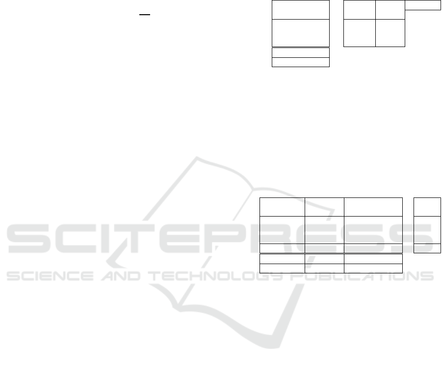
Table 1: Model of the three products problem.
P1 P2 P3
RHS Price
Total
b
udge
t
R1 2 0 1 ≤ 25 5 206
R2 1 1 1 ≤ 20 3
C1 1 ≥ 10 1
C2 1 ≥ 3 1
C3 1 ≥ 4 2
L. costs 1 1 8 MIN
Profi
t
236 MAX
Ideal values of objective functions of this model
are in the vector
65;45
.
1) Model Reformulation.
The model is reformulated using 5 unknown variables
,…,
representing unknow values of capacities
and requirements while respecting budget . The new
formulation of model is in Table 2.
Table 2: Reformulated model.
P1 P2 P3
y
R1
y
R2
y
C1
y
C2
y
C3
R1
2 0 1 -1 0 0 0 0
=
0
R2
1 1 1 0 -1 0 0 0
=
0
C1
1 0 0 0 0 -1 0 0
=
0
C2
0 1 0 0 0 0 -1 0
=
0
C3
0 0 1 0 0 0 0 -1
=
0
Budget
0 0 0 5 3 1 1 2
=
206
L. cost
1 1 8 0 0 0 0 0 MIN
Profit
2 3 6 0 0 0 0 0 MAX
2) Partial Optimization.
Ideal solutions are found solving two single objective
optimization models received by reformulation of the
initial model according to the (15).
The solution of minimization of the labour cost is
to produce only 14.71 pcs of the product P1 with
necessary 29.43 units of resource 1 and 14.71 units of
resource 2. This system design allows to closed only
the first contract. The minimal labour cost is 14.71
thous. CZK and maximal profit is 29.43 thous. CZK.
The solution of maximization of the profit is to
produce only 51.5 pcs of the product P2 with
necessary 51.5 units of resource 2. This system design
allows to closed only the second contract. The
minimal labour cost is 154.5 thous. CZK and
maximal profit is 51.5 thous. CZK.
Ideal values of objective functions under budget
are in the vector
14.71;154.5
.
3) Metaoptimization.
Based on the ideal and nadir objective function values
the following weights are used for calculation of
metaoptimization model (Table 3)
ICORES 2019 - 8th International Conference on Operations Research and Enterprise Systems
478
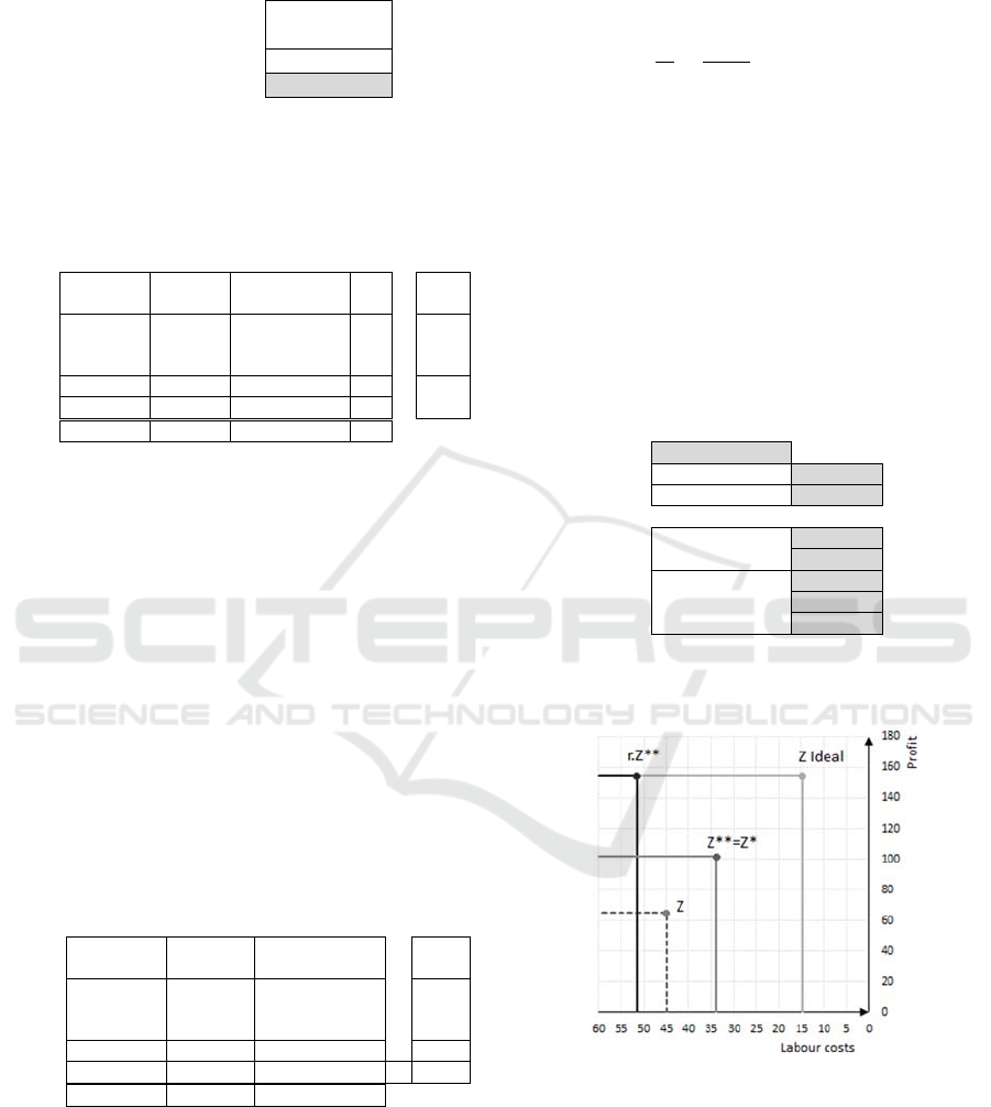
Table 3: Normalized weights.
Cost Profit
14.71 154.5
51.5 29.43
Average 33.11 91.96
Normalized weights 0.73 0.27
The formulation of the metaoptimization model
minimizing the deviation of ideal values is in Table 4.
Table 4: Formulation and solution of metaoptimization
model.
P1 P2 P3 yR1 yR2 yC1 yC2 yC3
R1
2 0 1 -1 0 0 0 0 0 = 0
R2
1 1 1 0 -1 0 0 0 0 = 0
C1
1 0 0 0 0 -1 0 0 0 = 0
C2
0 1 0 0 0 0 -1 0 0 = 0
C3
0 0 1 0 0 0 0 -1 0 = 0
L. cost
1 1 8 0 0 0 0 0 -1.4 = 14.7
Profit
2 3 6 0 0 0 0 0 3.8 = 154.5
Dev.
0 0 0 0 0 0 0 0 1 MIN
Its optimal solution is to produce only 33.82 pcs
of the product P2 with necessary 33.8 units of
resource 2. This system design allows to closed only
the second contract. The minimal labour cost is 33.82
thous. CZK and maximal profit is 101.44 thous. CZK.
The vector
∗
is
33.82;101.44
4) Metametaoptimization.
With the best obtainable values of both criteria is
solved the metametamodel to find the minimal
necessary budget. Similarly, as in the STEP method,
the decision maker could change these values and
repeat the metamodel optimization from the previous
step. Now the minimal budget is calculated with
objective functions values of the optimal solution of
metaoptimization model (Table 5).
Table 5: Metametaoptimization model.
P1 P2 P3
y
R1
y
R2
y
C1
y
C2
y
C3
R1
2 0 1 -1 0 0 0 0
=
0
R2
1 1 1 0 -1 0 0 0
=
0
C1
1 0 0 0 0 -1 0 0
=
0
C2
0 1 0 0 0 0 -1 0
=
0
C3
0 0 1 0 0 0 0 -1
=
0
L. cost
1 1 8 0 0 0 0 0 ≤ 33.8
Profit
2 3 6 0 0 0 0 0 ≥ 101.4
Budget
0 0 0 5 3 1 1 2 MIN
The optimal solution of metametaoptimization
model is equal to the solution of the previous
metaoptimization model, so we receive
∗∗
∗
33.82;101.44
. The minimal necessary budget
is
135.26 thous. CZK, what is less then we suppose to
invest to production. So, it is possible to extend the
production process.
4) Optimal System Design.
Optimal production structure under optimal design of
production system and available budget allows
expansion according to the optimal path ratio which
is equal to
∗
.
1,523.
The optimal system design (Table 6) allows
producing 51.5 pcs of the product P2 with necessary
51.5 units of resource 2. This system design allows to
closed only the second contract on 51.5 pcs of
products of products sold. The minimal labour cost is
51.5 thous. CZK and maximal profit is 154.5 thous.
CZK;
∗∗
51.5;154.5
. This means that there is
no need for resource 1 but higher consumption of
resource 2, e. g. 51.5 units. Also, there is only one
optimal contract, the contract C2 with 51.5 pcs of
product 2.
Table 6: Optimal system design.
P1 P2 P3
0 51.5 0 Solution
L. costs 118 51.5
Revenue 2 3 6 154.5
Inpu
t
data
Resource R1 2 0 1 0 25
Resource R2 1 1 1 51.5 20
Contracts C1 1 0 0 0 10
Contracts C2 0 1 0 51.5 3
Contracts C3 0 0 1 0 4
In the figure 1 the objective functions values of
selected models are shown.
Figure 1: Values of labour costs and profit for selected
solutions of three products problem.
It is possible to say, that the optimal system design
has resulted in significantly higher profit but with the
highest labour cost. Optimal system design results in
necessity to product only one type of product and
allocate the whole budget for the second resource and
the contract for the optimal type of products.
Optimal Design of Production Systems: Metaoptimization with Generalized De Novo Programming
479

6 CONCLUSIONS
In this paper, we continued our previous discussion of
De Novo Programming; see Vlach and Brožová
(2018). We briefly recalled the original approach of
Zelený, rectified some oversights in the alternative
proposal by Shi. Then we presented adaptation of De
Novo methodology for models with capacity,
requirement, and balance constraints, where the
transformation to continuous knapsack problem is not
possible.
Our proposal for Generalized De Novo
Programing is a way to optimize the system design in
more general settings. In particular, it is possible to
deal with more types of constraints and more types of
criteria.
REFERENCES
Babic, Z., Pavic, I., 1996. Multicriterial production
planning by De Novo programming approach.
International Journal of Production Economics, 43(1),
59–66.
Benayoun, R., de Montgolfier, J., Tergny, J., 1971. Linear
Programming with Multiple Objective Functions:
STEP Method (STEM). Mathematical Programming 1,
366-375.
Vlach, M., Brožová, H., 2018. Remarks on De Novo
approach to multiple criteria optimization. In:
Proceedings of the 36th Conference on Mathematical
Methods in Economics. Prague: Faculty of
Management, University of Economics, 618-623.
Fiala, P., 2011. Multiobjective De Novo Linear
Programming. Acta Univ. Palacki. Olomuc., Fac. rer.
nat., Mathematica, 50(2), 29–36.
Huang, Ch.Y., Tzeng, G.H., 2007. Post-Merger High
Technology R&D Human Resources Optimization
through the De Novo Perspective. In: Advances in
Multiple Criteria Decision Making and Human Systems
Management: Knowledge and Wisdom, Ed. Y. Shi et
al., IOS Press, 47-64.
Gigch, J.P., 1991. System Design Modeling and
Metamodeling. Plenum Press: New York and London.
Roostaee, R. Izadikhah, M. Hosseinzadeh Lotfi F., 2012.
An Interactive Procedure to Solve Multi-Objective
Decision-Making Problem: An Improvement to STEM
Method, Journal of Applied Mathematics [online].
Accessible from: https://www.hindawi.com/journals/
jam/2012/324712/.
Shi, Y., 1995. Studies on Optimum-Path Ratios in De Novo
Programming Problems. Computers and Mathematics
with Applications, 29(5), 43–50.
Zelený, M., 2010. Multiobjective Optimization, Systems
Design and De Novo Programming. In: Zopounidis C.,
Pardalos P. M. (eds.): Handbook of Multicriteria
Analysis, Berlin: Springer.
Zelený, M., 2005. The Evolution of Optimality: De Novo
Programming. In: Proceedings of EMO 2005, LNC
3410, ed. C.A. Coello Coello et al., Springer-Verlag,
Berlin-Heidelberg, 1-13.
Zelený, M., 1990a. De Novo Programming. Ekonomicko-
matematický obzor, 26(4), 406–413.
Zelený, M., 1990b. Optimal Given System vs. Designing
Optimal System: The De Novo Programming
Approach. International Journal of General System,
17(4), 295–307.
Zelený, M., 1986. Optimal system design with multiple
criteria: De Novo programming approach. Engi-
neering Costs and Production Economics, 10(2), 89-94.
Zhang, Y. M., Huang, G. H., Zhang, X. D., 2009. Inexact
de Novo programming for water resources systems
planning. European Journal of Operational Research,
199, 531–541.
Zhuang, Z.Y., Hocine, A. 2018. Meta goal programing
approach for solving multi-criteria de Novo programing
problem. European Journal of Operational Research,
265, 228–238.
ICORES 2019 - 8th International Conference on Operations Research and Enterprise Systems
480
