Understanding of Non-linear Parametric Regression and Classiﬁcation

Models: A Taylor Series based Approach

Thomas Bocklitz

1,2

IPC Junior Research Group ’Statistical Modelling and Image Analysis’,

Institute of Physical Chemistry and Abbe Center of Photonics (IPC), Friedrich-Schiller-University, Jena, Germany

IPHT Working Group ’Statistical Modelling and Image Analysis’, Leibniz Institute of Photonic Technology (IPHT),

Jena, Germany

Keywords:

Non-linear Models, Taylor Series, Model Approximation, Model Interpretation.

Abstract:

Machine learning methods like classiﬁcation and regression models are speciﬁc solutions for pattern recog-

nition problems. Subsequently, the patterns ’found’ by these methods can be used either in an exploration

manner or the model converts the patterns into discriminative values or regression predictions. In both ap-

plication scenarios it is important to visualize the data-basis of the model, because this unravels the patterns.

In case of linear classiﬁers or linear regression models the task is straight forward, because the model is

characterized by a vector which acts as variable weighting and can be visualized. For non-linear models the

visualization task is not solved yet and therefore these models act as ’black box’ systems. In this contribu-

tion we present a framework, which approximates a given trained parametric model (either classiﬁcation or

regression model) by a series of polynomial models derived from a Taylor expansion of the original non-linear

model’s output function. These polynomial models can be visualized until the second order and subsequently

interpreted. This visualization opens the ways to understand the data basis of a trained non-linear model and

it allows estimating the degree of its non-linearity. By doing so the framework helps to understand non-linear

models used for pattern recognition tasks and unravel patterns these methods were using for their predictions.

1 INTRODUCTION

Pattern recognition is an emerging ﬁeld, which ﬁnds

numerous applications in a wide range of other scien-

tiﬁc ﬁelds, e.g. in biology and chemistry (de S

a, 2001;

Bishop, 2011). In these both application ﬁelds the

aim is to extract useful information like patterns out

of high dimensional datasets from chemical and bio-

logical experiments (Bocklitz et al., 2014b). In these

application ﬁelds often supervised machine learning

methods like classiﬁcation or regression approaches

are used to analyze un-targeted higher-dimensional

measurements, like images (Bocklitz et al., 2014a),

spectra (Kemmler et al., 2010; Bocklitz et al., 2009)

or time traces (Volna et al., 2016).

If the classiﬁcation or regression task, which

should be solved, is complicated, non-linear models

are advisable. Because of the fact that biological or

chemical pattern recognition tasks are typically hard

to solve, non-linear models must be applied. Never-

theless, a drawback of these non-linear models is that

the patterns, which the model learned, cannot be ex-

tracted and visualized easily. In this way non-linear

classiﬁcation and regression models work as ’black

box’ methods and no insight in their working wise

can be gained. This is a drastic drawback of these

non-linear methods, because in the application sci-

ence always an interpretation of the model is needed.

Such an interpretation would allow to gain new in-

sights into the classiﬁcation task or regression task,

unravel pattern in the data and allow a check if the

model was learning artifacts.

To solve this interpretation task two schemes were

developed. One scheme is the calculation of variable

importance measures, like Gini importance or permu-

tation importance (Hapfelmeier et al., 2014), and the

other scheme is the visualization of instances, which

lead to an extreme prediction. Both workﬂows are

not optimal, because the variable importance do not

state, why and how a speciﬁc variable is utilized to

calculate quantitatively the output. Therefore, a direct

model interpretation approach is needed, which lead

to a direct understanding of the non-linear model. A

solution for this issue is presented in this article.

The outline of this contribution is as follows. In

section 2 the Taylor series and parametric models

874

Bocklitz, T.

Understanding of Non-linear Parametric Regression and Classiﬁcation Models: A Taylor Series based Approach.

DOI: 10.5220/0007682008740880

In Proceedings of the 8th International Conference on Pattern Recognition Applications and Methods (ICPRAM 2019), pages 874-880

ISBN: 978-989-758-351-3

like classiﬁcation and regression techniques are intro-

duced. In section 3 our approximation scheme is pre-

sented and in section 4 the example datasets together

with the interpretation of the approximation models

with respect to the data are discussed. In section 5 the

paper is summarized and an outlook is given.

2 THEORETICAL

CONSIDERATIONS

2.1 Taylor Series

In this paragraph the Taylor series or Taylor expan-

sion is introduced. A Taylor series represents a given

function f : R 7→ R as an inﬁnite sum of terms that can

be calculated in a small neighborhood around a given

point x

(0)

∈ R. These terms contain the values of the

function’s derivatives at the point x

(0)

and this point is

called expansion point. If the inﬁnite sum is used and

it converges, the function and its Taylor series can be

used interchangeable

. If only ﬁnite terms of its Tay-

lor series are utilized an approximation of the function

f can be extracted. Then the Taylor’s theorem states

an estimate of the error such an approximation is fea-

turing. The polynomial formed by taking some initial

terms of the Taylor series is called a Taylor polyno-

mial and we will stick to this term through the arti-

cle. In Figure 1 Taylor polynomials of two different

exponentials are given, which were calculated at two

different expansion points. In the upper exponential

second order polynomials are used for approximation,

while in the lower trace linear approximations were

tested. It is clear that the Taylor polynomials approxi-

mate the function in a neighborhood of the expansion

point x

(0)

quite well. The error of the approximation

can be calculated via different error formulas related

to the polynomials, which were not used in the ap-

proximation.

In the further cause of the article we need to work

with high dimensional functions, which map from the

to the real numbers and we will denote the cor-

responding function with F : R

7→ R. We will de-

note the points of the R

in bold: x ∈ R. The expan-

sion point is again termed x

(0)

∈ R. The Taylor series

can be calculated using the higher dimensional deriva-

tives, e.g. Gradient and Hessian. The corresponding

Taylor series (Bronstein et al., 2012) can be expressed

as:

The function needs to be an analytical function that this

equality holds true (Bronstein et al., 2012).

0 1 2 3 4 5

0 50 100 150

exponential increase

1. order approximation

2. order approximation

Figure 1: One-dimensional Taylor expansion. Linear and

quadratic approximations of two exponential functions in

two different expansion points are shown. In the neighbor-

hood of the expansion point the approximation quality is

appropriate.

F (x) = T

(0)

(x) =

∞

∑

i=0



x − x

(0)



· ∇

(0)

. (1)

If only the constant and linear term is used a Taylor

polynomial approximation results, which can be writ-

ten as follows:

F (x) ≈ T

(1)

(0)

(x) = F



(0)





x − x

(0)



· ∇F|

(0)

. (2)

If the quadratic term is added, a quadratic Taylor ap-

proximation is generated and can be written as:

F (x) ≈ T

(2)

(0)

(x) = T

(1)

(0)

(x)



x − x

(0)



· ∇

(0)



x − x

(0)



. (3)

In this ways the function F can be approximated by

a quadratic function using only the values around the

expansion point x

(0)

2.2 Parametric Classiﬁcation and

Regression Models

Two important groups of machine learning methods

used for pattern recognition tasks are classiﬁcation

and regression models. Parametric models form an

important sup-group of these models and they learn

an output function, e.g. the parameters of this output

function, based on a given training dataset. Typically

this learning involves the solving of an optimization

problem in the training phase of the algorithm. After

Understanding of Non-linear Parametric Regression and Classiﬁcation Models: A Taylor Series based Approach

875

this procedure is ﬁnished, the output function:

F : R

7→ R (4)

is ﬁxed and can be used for prediction of new mea-

surements or instances. The prediction can be done

directly (in the case of regression models) or after the

application of a threshold to the output function to

form a class decision in case of classiﬁcation models.

To derive different machine learning methods differ-

ent optimization problems are stated and in turn they

lead to different output functions. The output func-

tions have in common that certain parameters are cho-

sen beforehand (hyper-parameters) and other parame-

ters are optimized or estimated based on the trainings

dataset. Mathematically, this yields to the fact that

the output function is parametrized F (x;p,q). Some

of the parameters, e.g. the hyper-parameters q, are

ﬁxed before training, while other parameters p have

to be determined in the trainings procedure based on

a given training dataset.

In the following, three examples of output func-

tions are given together with their parameters. The

output function of Fisher’s linear discriminant anal-

ysis (LDA) (Fisher, 1936), Vapnik’s support vector

machines (SVM) (Cortes and Vapnik, 1995) and ar-

tiﬁcial neural networks

(ANN) (Bishop, 1995) are

set together in the Equation 5 to 7. Due to its linear-

ity the output function of the LDA can be written as

scalar product with a learned vector s:

F (x) = (x · s) . (5)

The output of the LDA’s output function is subse-

quently converted via a threshold into a class predic-

tion. In contrast the output function of a SVM reads

as follows:

F (x) =

∑

i=1



(i)



+ b

. (6)

While the number of support vectors i ∈

{

1,··· ,N

}

the coefﬁcients α

and the value b are optimized, the

kernel function K is choose beforehand. Depending

on the chosen kernel K the SVM is a linear classiﬁer

or a non-linear classiﬁer. Another often applied re-

gression and classiﬁcation model is the ANN and its

output function can be written as follows:

F (x) = f

∑

j=1

1 j

∑

i=1

+ w

. (7)

In this formula f , f

are the activation functions of

hidden and output layer. The number of neurons are

Here, we restrict ourselves to three layer feed forward

networks with one output neuron, but the generalization to

different topologies is straight forward.

n,n

. These values are the hyper-parameter, while the

weights w

1 j

and the biases w

1 j

are learned.

These latter parameters are optimized while training

to minimize the summed error of all trainings in-

stances E =

∑

i=1

. The error of every individual

pattern is back propagated from layer to layer and

the derivatives of the error function with respect to

the weights and biases in the network is calculated

(Bishop, 1995; Rumelhart et al., 1986). Finally, the

weights and biases are updated accordingly.

3 PROPOSED METHOD

In order to get an insight into the patterns a non-

linear model is used for prediction, we combine the

aforementioned two concepts. Basically we generate

a quadratic approximation of the non-linear machine

learning model (regression or classiﬁcation model),

which was initially used for pattern recognition. We

utilized a Taylor polynomial until the second order

(see Equation 3). If the linear part of the second order

Taylor polynomial is explicitly written, it looks like



x − x

(0)



· ∇F|

(0)

(8)

∑

i=1



− x

(0)



· ∇



(0)



and can be understood as a variable weighting. The

value of the Gradient ∇F|

(0)

represents the weight

of the variables. The Equation 8 is similar to output

function of the LDA (Equation 5). A similar interpre-

tation as for the Gradient holds true for the quadratic

term and it reads (without the 1/2 factor)



x − x

(0)



∇

(0)



x − x

(0)



(9)

∑

i=1

∑

j=1



− x

(0)





∇

(0)



i, j



− x

(0)



The advantage of this approximation is that we can

quantify the degree of non-linearity of the original

non-linear model by comparing the prediction of the

original model with the predictions of approximations

with different degree. If the prediction of an approx-

imation is worse compared with the original model,

the non-linearity is at least higher as the approxima-

tion degree n. This fact results from the Taylor’s rest

formula, which state that the rest term is





x − x

(0)



(n+1)



. (10)

If the approximation performance in terms of the

model prediction, e.g. either accuracy or Root-Mean-

Squared-Error (RMSE), is acceptable, the approxima-

tion can be used instead of the original model. The

ICPRAM 2019 - 8th International Conference on Pattern Recognition Applications and Methods

876

range of acceptable performance of the model can

only be discussed in terms of the application scenario

and is not further discussed here. If only a model up

to the second order is needed, e.g. its performance is

sufﬁcient, the quadratic part and the linear part of the

model can be visualized and subsequently interpreted.

The visualization of the approximation can be done

by plotting the Gradient of the model, e.g. the lin-

ear part of the approximation, and the Hessian, e.g.

the quadratic part of the approximation, in false col-

ors. The Gradient can be interpreted due to Equation 2

and Equation 8 as a variable weighting. Additionally,

the sign and its magnitude can be interpreted, which

is an advantage over any variable importance score.

Beside this linear part of the approximation also the

quadratic part, e.g. the Hessian, can be visualized and

interpreted. Due to Equation 3 and Equation 9 the val-

ues of the Hessian on the main diagonal correspond

to pure quadratic dependencies of the output function

on the respective variable, while the off-diagonal ele-

ments belong to dependencies of the output function

on variable combinations. The magnitude and sign of

the Hessian values can be interpreted in a similar way

as above for the Gradient.

4 EXPERIMENTAL RESULTS

AND DISCUSSIONS

4.1 Datasets

We utilized two datasets respectively models to

demonstrate the developed approximation frame-

work. We used a low dimensional dataset for the

demonstration of the approximation of classiﬁcation

models and a high dimensional dataset for the demon-

stration of the approximation of regression models.

The classiﬁcation will be demonstrated on a sub-

set of Fisher’s Iris ﬂower dataset (Fisher, 1936) and

we used the version shipped with the R package

’MASS’ (Venables and Ripley, 2002). This dataset

consist of 4 variables (the length and the width of the

sepals and petals, in centimeters) to discriminate three

species of Iris (Iris setosa, Iris virginica and Iris ver-

sicolor). We removed the species Iris setosa from the

dataset to form a binary classiﬁcation task. We solved

this classiﬁcation task using a 3-layer feed-forward

artiﬁcial neural network implemented using the ’nnet’

package (Venables and Ripley, 2002), which is called

Iris-ANN from here on. The hyper-parameters were a

quadratic error function, a linear output of the output

layer and there were 4 input neurons, 2 hidden neu-

rons and one output neuron. The group Iris virginica

5 10 15 20 25 30

5 10 15 20 25 30 35

x/µm

y/µm

−0.1

0.0

0.1

0.2

0.3

0.4

0.5

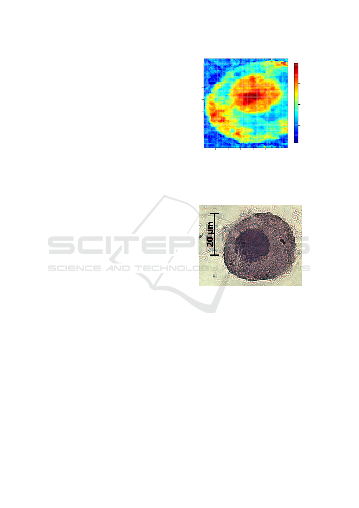
Figure 2: Output of the DNA-ANN for an examples cell.

The output of the DNA-ANN, which was trained based on

Raman spectral scans of cells, is shown. The visual ap-

pearance of the result indicated that the nucleus region is

highlighted.

Figure 3: HE image of an example cell. The staining of the

cell after Raman spectroscopic measurement was the only

validation of the DNA-ANN’s output.

was coded with 1, while the group Iris versicolor was

coded with 0.

The dataset and model used to demonstrate the

approximation of a regression model was published

in reference (Bocklitz et al., 2009). In this publica-

tion a ANN was trained to highlight the cell nucleus

and the model is called DNA-ANN from here on. It

was trained using Raman spectra of cells exhibiting a

strong DNA/RNA contribution. The model was using

a principal component analysis (PCA) for dimension

reduction to 60 PCs, which were used for training the

DNA-ANN. Ten hidden neurons and on linear out-

put neuron were utilized. The validation in reference

(Bocklitz et al., 2009) was done based on visual com-

parison of the output of the DNA-ANN (Figure 2)

with images of Hematoxylin and Eosin stained cells

(Figure 3). The question arose, which patterns in the

spectroscopic data, e.g. Raman bands, were used to

Understanding of Non-linear Parametric Regression and Classiﬁcation Models: A Taylor Series based Approach

877

calculate the DNA-ANN output. With this informa-

tion the model could be understand and the Figure 2

can be interpreted accordingly.

4.2 Software

All computations were done in the free programming

environment R using the packages ’MASS’, ’nnet’

and ’numDeriv’.

4.3 Results – Classiﬁcation Technique

In order to approximate a given classiﬁer we ﬁrst

trained an ANN based on the Iris dataset with only

one output neuron (Iris-ANN). The coefﬁcients of the

approximation of the Iris-ANN are calculated using

Equation 3. Here the trained Iris-ANN was approxi-

mated by a second order Taylor polynomial T

(2)

(0)

(x),

which was expanded around the mean of the reduced

Iris dataset (see Equation 12). We also substitute the

difference x − x

(0)

by ∆x:

∆x = x − x

(0)

. (11)

For the reduced Iris data set this equation reads as fol-

lows:

∆x = x −







6.262

2.872

4.906

1.676







sepal length

sepal width

petal length

petal width

. (12)

In order to extract the Gradient and the Hessian from

the given non-linear model two possibilities arise.

First, the analytical derivatives or numerical estimates

of the derivatives can be utilized. Both methods are

suitable, but care has to be taken to include the dimen-

sional reduction, converting functions and/or scaling

steps, if the analytical formulas are used. The nu-

merical derivatives already include all three steps,

therefore we utilized the numerical approach (Gilbert,

2006).

The approximation of the Iris-ANN is called P

(2)

Iris

for

clarity reasons. The corresponding coefﬁcients of the

approximation P

(2)

Iris

are given in Equation 13:

(2)

Iris

(∆x) = 0.46 +







−1.82

−3.12

5.17

6.29







· ∆x (13)

∆x







0.98 1.56 −2.54 −3.35

1.56 2.89 −4.26 −5.74

−2.54 −4.26 7.23 5.47

−3.35 −5.74 5.47 11.42







∆x .

The classiﬁcation results on the training dataset are

summarized in Table 1 for the Iris-ANN and in Ta-

ble 2 for the approximation P

(2)

Iris

. The results of the

classiﬁer P

(2)

Iris

(5 errors) are not as exact as the results

of the Iris-ANN (1 error), but the P

(2)

Iris

approximation

is interpretable and features only a low degree of non-

linearity. From the Gradient values (Equation 13) it is

clear that an increased sepal length and width is an in-

dicator for Iris versicolor, because it was coded with

zero in the trainings phase. Petal length and width

are linear important for the Iris virginica group. The

Hessian can be interpreted in the same manner. All

variables are quadratically linked to the Iris virginica

group, while combination of variables are negatively

correlated with the Iris virginica group. The large er-

ror rate might be attributed to a higher degree of non-

linearity of the Iris-ANN or that the Iris-ANN features

less parameter compared to the P

(2)

Iris

approximation.

Table 1: Confusion table of the Iris-ANN model.

predicted

classes true classes

versicolor virginica

versicolor 49 0

virginica 1 50

Table 2: Confusion table of the P

(2)

Iris

model.

predicted

classes true classes

versicolor virginica

versicolor 45 0

virginica 5 50

4.4 Results – Regression Technique

To prove the approximations and visualization ap-

proach for regression techniques, we also performed

a second order approximation of the described DNA-

ANN model published in (Bocklitz et al., 2009).

The expansion point was the dataset mean and we

termed the second order approximation P

(2)

DNA

. First,

we checked the quality of the approximation. To do

so, we compared the output of the DNA-ANN with

the output of the P

(2)

DNA

approximation. We visualized

both outputs in Figure 4. The output of both models

was sorted according to the DNA-ANN output, which

forms a sigmoidal shaped curve. The difference be-

tween both outputs is given in green at the bottom of

Figure 4. It can be seen at the edges around 0 and

around 8000, that only for extreme values a larger er-

ICPRAM 2019 - 8th International Conference on Pattern Recognition Applications and Methods

878

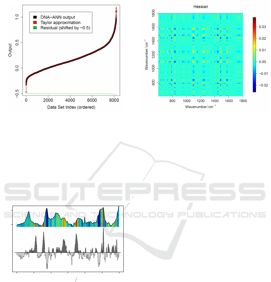
Figure 4: DNA-ANN output and approximation output.

The DNA-ANN output is visualized together with the out-

put of the P

(2)

DNA

approximation. In the lower part the differ-

ence of both outputs is plotted. The approximation quality

is good as the RMSE is only 0.0019.

ror between the DNA-ANN output and the P

(2)

DNA

out-

put exists. In this case the RMSE of the approxima-

tion was 0.0019. Therefore, the second order approx-

imation is sufﬁcient to approximate the (given) DNA-

ANN model in an appropriate manner.

1800 1600 1400 1200 1000 800 600

Linear part of the approximation

Wavenumber cm

−1

Normalized Raman Intensity

0.01 0.06

−

Figure 5: Gradient ∇F|

−→

of the DNA-ANN and mean of

the dataset. The values of the Gradient are visualized in the

lower panel and they can be interpreted: positive features

in the Gradient mark areas which are connected quantita-

tively with a positive output of the DNA-ANN, e.g. a higher

DNA content. The spectrum in the upper panel represents

the dataset mean and the false-colors show the Gradient val-

ues.

Due to the low RMSE of only 0.0019, the

quadratic approximation can be used instead of the

original non-linear regression model. Because it is

composed of a linear and a quadratic part in a sum,

we can investigate the linear and quadratic behavior

separately. The linear part of the approximation is

Figure 6: Hessian ∇

−→

of the DNA-ANN. Again the

positive areas mark variable combinations which are corre-

lating with a higher DNA-ANN output, while negative areas

mark the opposite.

plotted in Figure 5. This ﬁgure is composed of the

mean (upper panel) and the Gradient (lower panel).

The false color within the mean (upper panel) repre-

sents again the values of the Gradient. Positive values

in the Gradient can be interpreted that they are posi-

tively contributing to the model’s output with its value

as weight. Negative values are negatively used within

the output of the model. For example the sharp feature

at 785 cm

−1

marks a vibration of DNA/RNA and this

feature is positively correlated with the DNA-ANN’s

output, which indicate a correct interpretation of the

DNA-ANN.

The quadratic term can be also interpreted. The Hes-

sian is visualized in Figure 6 and its interpretation

can be done like in the case of the classiﬁer above.

A positive or negative value on the main diagonal

means that the quadratic value of the corresponding

variable is positively or negatively connected with the

output of the DNA-ANN. This connection strength

is represented by the value itself. An off-diagonal

value is linked with variable combinations, which

then characterizes a positive or negative output, de-

pending on the sign (and magnitude) of the Hessian

value at the speciﬁc off-diagonal position. This in-

terpretation goes beyond variable/feature importance

measures, because the magnitude of the variable’s in-

ﬂuence on the output is estimated and can be sub-

sequently interpreted. This interpretation possibility

leads to an understanding of the DNA-ANN.

Understanding of Non-linear Parametric Regression and Classiﬁcation Models: A Taylor Series based Approach

879

5 CONCLUSION

In this contribution we presented a framework, which

allows the interpretation of patterns in the data, which

a parametric non-linear classiﬁcation or regression

model was using for modeling. This framework is

working based on a Taylor expansion of the learned

output function of the respective model. This expan-

sion leads to a series of polynomial models (classi-

ﬁers, regressors), which can be used to understand

the non-linearity of a given non-linear model. A fur-

ther advantage of these polynomial approximations is

the fact that the linear and quadratic part can be vi-

sualized. By doing so, patterns in the data, which

were used in the modeling by the non-linear model,

can be elucidated. This approach can be used to ex-

tract, which variable or variable combinations are im-

portant to predict a special class or which are posi-

tively/negatively connected with the output of a re-

gression model. Nevertheless, the interpretation goes

beyond, because the magnitude of the variable inﬂu-

ence on the output is estimated and can be interpreted.

This interpretation possibility is advancement over

variable/feature importance measures, which only in-

dicate important variables but not their speciﬁc, quan-

titative inﬂuence on the output. With this framework

non-linear models can be understood and they are not

working as ’black box’ systems anymore.

ACKNOWLEDGEMENTS

The funding of the Leibniz association via the

ScienceCampus ’InfectoOptics’ for the project

’BLOODi’, the funding of the DFG for the project

’BO 4700/1’ and funding of the BMBF for the

project URO-MDD (FKZ 03ZZ0444J) are highly

appreciated.

REFERENCES

Bishop, C. M. (1995). Neural Network for Pattern Recog-

nition. Clarendon Press.

Bishop, C. M. (2011). Pattern Recognition and Ma-

chine Learning. Information Science and Statistics.

Springer.

Bocklitz, T., K

ammer, E., St

ockel, S., Cialla-May, D., We-

ber, K., Zell, R., Deckert, V., and Popp, J. (2014a).

Single virus detection by means of atomic force mi-

croscopy in combination with advanced image analy-

sis. J. Struct. Biol., 188(1):30–38.

Bocklitz, T., Putsche, M., St

uber, C., K

as, J., Niendorf,

A., R

osch, P., and Popp, J. (2009). A comprehensive

study of classiﬁcation methods for medical diagnosis.

J. Raman Spectrosc., 40:1759–1765.

Bocklitz, T., Schmitt, M., and Popp, J. (2014b). Ex-vivo and

In-vivo Optical Molecular Pathology, chapter Image

Processing – Chemometric Approaches to Analyze

Optical Molecular Images, pages 215–248. Wiley-

VCH Verlag GmbH & Co. KGaA.

Bronstein, I. N., Hromkovic, J., Luderer, B., Schwarz, H.-

R., Blath, J., Schied, A., Dempe, S., Wanka, G., and

Gottwald, S. (2012). Taschenbuch der mathematik,

volume 1. Springer-Verlag.

Cortes, C. and Vapnik, V. (1995). Support-Vector Networks.

Machine Learning, 20(3):273–297.

de S

a, J. P. M. (2001). Pattern Recognition. Springer.

Fisher, R. A. (1936). The use of multiple measurements in

taxonomic problems. Annals Eugen., 7:179–188.

Gilbert, P. (2006). numDeriv: Accurate Numerical Deriva-

tives. R package version 2006.4-1.

Hapfelmeier, A., Hothorn, T., Ulm, K., and Strobl, C.

(2014). A new variable importance measure for ran-

dom forests with missing data. Statistics and Comput-

ing, 24(1):21–34.

Kemmler, M., Denzler, J., R

osch, P., and Popp, J. (2010).

Classiﬁcation of microorganisms via raman spec-

troscopy using gaussian processes. Pattern Recogni-

tion, online:81–90.

Rumelhart, D. E., Hinton, G. E., and Williams, R. J. (1986).

Learning representations by back-propagating errors.

Nature, 323:533–536.

Venables, W. N. and Ripley, B. D. (2002). Modern Applied

Statistics with S. Springer, New York, fourth edition.

Volna, E., Kotyrba, M., and Janosek, M. (2016). Pattern

Recognition and Classiﬁcation in Time Series Data.

IGI Global.

ICPRAM 2019 - 8th International Conference on Pattern Recognition Applications and Methods

880