Dynamic Vehicle Routing under Uncertain Travel Costs and Refueling

Opportunities

Giorgos Polychronis and Spyros Lalis

Department of Electrical and Computer Engineering, University of Thessaly, Volos, Greece

Keywords:

Traveling Salesman Problem, Vehicle Routing Problem, Uncertainty, Dynamic Route Planning.

Abstract:

We study the vehicle routing problem for a system where there is some uncertainty regarding both the cost of

travel and the refueling opportunities. Travel cost stands for the energy spent by the vehicle to move between

locations. Refueling opportunities are offered at known locations where the vehicle can harvest or re-gain

some of the lost energy. The objective is to visit a set of predeﬁned locations without exhausting the energy

of the vehicle. We describe the problem in a formal way, and propose a heuristic algorithm for taking routing

decisions at runtime. We evaluate the algorithm for a grid topology as a function of the number of locations to

be visited and the autonomy degree of the vehicle, showing that the proposed algorithm achieves good results

as long as the energy margins are not very tight.

1 INTRODUCTION

Unmanned Vehicles (UVs) will play a major role

in next-generation applications. In particular, Un-

manned Aerial Vehicles (UAVs) are already being

used in the domain of agriculture and surveillance.

Other types of UVs, such as Unmanned Ground Ve-

hicles (UGVs) or Unmanned Underwater Vehicles

(UUVs), though more exotic, are becoming more ma-

ture and affordable, and will most likely be used in

several applications in the future.

A typical scenario is for UVs to visit speciﬁc lo-

cations or entire areas in order to take measurements

or to detect objects / phenomena of interest. For ex-

ample, in agriculture, UVs scan a crop ﬁeld to detect

problematic spots that are infected with pests. Simi-

larly, in search and rescue missions, UVs scan a tar-

get area to ﬁnd missing persons. Yet another example

is for a UV to patrol an area by visiting several pre-

deﬁned locations. In all these cases, the UV should

perform the mission as efﬁciently as possible.

This problem is known as the Vehicle Routing

Problem (VRP), which in turn is an extension of the

Traveling Salesman Problem (TSP). In a nutshell, the

VRP consists in ﬁnding a travel plan that can be fol-

lowed by a vehicle in order to visit a set of target loca-

tions. The problem has been studied in many variants

and different constraints regarding the speciﬁc paths

that can be followed by the vehicle, the locations to

be visited or the time window where certain locations

have to be visited. Also, in several formulations, the

vehicle is assumed to have ﬁnite fuel/energy reserves

or serving capacity, which can be replenished by vis-

iting special so-called depot nodes.

In this paper, we investigate a variant of the VRP

where there is uncertainty regarding the cost of travel

and the energy harvesting / refueling opportunities

that can be exploited by the vehicle. Algorithms that

compute the travel plan based on static data are not

suitable in this case. This is because these plans may

turn out to be infeasible for the situation that the vehi-

cle faces during the mission — its energy reserves will

be depleted before completing the mission. Instead, a

more dynamic approach is required, so that routing

decisions can be taken and adjusted at runtime, based

on the situation at hand.

The main contributions of the paper are: (i) it pro-

vides a formal description for a new variant of the ve-

hicle routing problem; (ii) it proposes a heuristic algo-

rithm to tackle the problem; (iii) it evaluates the pro-

posed algorithm, showing that it performs well com-

pared to other static solutions of the problem.

The rest of the paper is structured as follows. Sec-

tion 2 gives an overview of related work. Section 3

describes the problem we study in a formal way. Sec-

tion 4 presents the algorithm for solving the problem.

Section 5 evaluates the algorithm for different scenar-

ios. Finally, Section 6 concludes the paper.

Polychronis, G. and Lalis, S.

Dynamic Vehicle Routing under Uncertain Travel Costs and Refueling Opportunities.

DOI: 10.5220/0007673900520063

In Proceedings of the 5th International Conference on Vehicle Technology and Intelligent Transport Systems (VEHITS 2019), pages 52-63

ISBN: 978-989-758-374-2

2 RELATED WORK

Different variants of the VRP and the TSP have been

investigated. We give a brief overview, and compare

with the problem we address in our work.

2.1 Vehicle Routing with Fuel/Energy

Constraints and Periodic Visits

In the so-called periodic vehicle routing problem and

multi-depot periodic vehicle routing problem (An-

gelelli and Speranza, 2002; Cordeau et al., 1997; Gau-

dioso and Paletta, 1992; Vidal et al., 2012; Alonso

et al., 2008; Rahimi-Vahed et al., 2013; Escobar et al.,

2014), the objective is to periodically visit a set of

destinations (target nodes) using one or more vehi-

cles. Vehicles have limited energy reserves and may

recharge/refuel at special depot stations. There are

more variations where the targets have different pri-

orities, vehicles have different capabilities/capacities,

and the targets must be visited within a time interval.

We brieﬂy discuss such work below.

Work in (Las Fargeas et al., 2012) investigates the

problems of persistent visitation with fuel constraints.

In this case, the vehicle perpetually visits the target

nodes (customer nodes), while each customer must

be visited at a speciﬁc rate. The fuel of the vehicle is

limited, so it is necessary to visit nodes with refueling

properties. The problem aims at satisfying the rate of

visit for each destination, as well as at minimizing the

total cost of fuel consumption.

The problem of continuous monitoring is studied

in (Mersheeva, 2015), where the mission is accom-

plished by several heterogeneous vehicles of different

types with limited resources. The objective is to visit

periodically a set of target nodes with different prior-

ities in a given time interval. The rate at which each

target node needs to be visited by any of the vehicles

is proportional to its priority. There is also a set of de-

pot nodes where vehicles can change their batteries,

however each type of vehicle requires a different type

of battery; only vehicles of the same type can use the

same type of battery. Also, the number of the different

types of batteries available at each depot is limited.

All the above formulations correspond to VRPs

with a ﬂeet of one or more vehicles that have en-

ergy/fuel limitations. Each edge of the graph is as-

sociated with a cost, and the energy of the vehicles

decreases accordingly based on that cost. There are

also one or more so-called depot nodes, where the ve-

hicles can refuel, fully or partially. The main goal is

to ﬁnd a path that minimizes the total cost of the mis-

sion, which is the sum of the costs of the edges chosen

to be used in the path of the vehicles. Another objec-

tive is to satisfy the visit rates of the target nodes.

The main difference between the above and our

work is that in our case the cost of travel between

nodes as well as the amount of energy/fuel that can

be gained at depot nodes, is not known a priori with

full certainty.

2.2 Vehicle Routing with Stochastic

Elements

The objective of vehicle routing problem with

stochastic demands is for a ﬂeet of one or more ve-

hicles, which have a ﬁnite serving capacity and may

also have fuel constraints, to visit and serve a set of

known target nodes (customers). However, the ex-

act demand of each customer is not known before-

hand. As a result, when a vehicle visits a customer,

it may ﬁnd out that the demand exceeds its remain-

ing capacity. The failure to properly service the cus-

tomer can be ignored, at a penalty, and the vehicle

may proceed to the next customer. Alternatively, the

vehicle may go to a depot node in order to acquire

the missing resources to restore its servicing capacity,

and then return to service the customer. This problem

is researched in many works (Bertsimas, 1992; Sec-

omandi, 2001; Laporte et al., 2002; Marinakis et al.,

2013; Rei et al., 2010; Juan et al., 2011; Marinaki and

Marinakis, 2016). Moreover, in (Erera et al., 2010)

and (Mendoza et al., 2016) the problem is investigated

for the more general case where the goal is to mini-

mize the travel time with the additional constraint of

keeping the travel time below a given upper bound.

In the vehicle routing problem with stochastic

travel times, a ﬂeet of one or more vehicles, which

may have capacity and/or fuel constraints, visit a set

of known targets, but in this case, the travel time is

a random variable. Also, each target has a time win-

dow during which it is available for visits by a vehi-

cle. If the target is not visited/served within that time

window, there is a penalty. The objective is to route

the vehicles so as to minimize the total penalty. Al-

gorithms tackling this problem are described in (Tas¸

et al., 2013; Laporte et al., 1992; Van Woensel et al.,

2003; Kenyon and Morton, 2003; Ehmke et al., 2015;

Miranda and Conceic¸

ao, 2016; Tas¸ et al., 2014).

The vehicle routing problem with stochastic cus-

tomers consists in using a ﬂeet of vehicles, which may

have capacity and/or fuel constraints, to visit a set of

target customers. However, these targets require a

visit only with some probability, thus a vehicle may

visit a node that does not need to be serviced. Indica-

tive work can be found in (Gendreau et al., 1996; Gen-

dreau et al., 1995; Bent and Van Hentenryck, 2004).

Dynamic Vehicle Routing under Uncertain Travel Costs and Refueling Opportunities

Our work is more similar to the VRP with stochas-

tic travel times. However, the main constraint there,

is the travel time, whereas in our work the main con-

straint is the energy of the vehicle, which can also in-

crease its energy reserves by visiting certain nodes. It

is also important to note that in our work the mission

ends when the vehicle exhausts its energy. This is a

major difference compared to the VRP with stochastic

demands, in which case the vehicle can always go to a

depot node in order to restore its capacity. As a conse-

quence, in our work, it is not always possible to visit

all nodes, in contrast to most other problem formu-

lations where this is always feasible and the problem

consists in minimizing the travel cost and/or time vio-

lation penalty. In this sense, our work is closer to (Er-

era et al., 2010) and (Mendoza et al., 2016), which

have a similar constraint for the travel cost. But in

our case the stochasticity concerns the travel cost and

energy gains, not the customer demands, and the ob-

jective is to maximize the number of target nodes that

are visited by the vehicle.

2.3 Energy-efﬁcient Path Planning

Several algorithms have been designed to compute an

energy-efﬁcient route between two nodes, based on

an abstract graph where the weights at edges repre-

sent the energy consumption or the energy restoration.

The difference to a typical shortest-path algorithm is

that the computed routes minimize the sum of edge

costs, not the number of edges. For instance, (Sachen-

bacher et al., 2011) deals with the problem of energy-

efﬁciency as a special case of the constrained short-

est path problem, while in (Artmeier et al., 2010) the

problem of energy-efﬁcient path planning is viewed

as a cost minimization problem. In both cases, the

ability of the vehicle to gain energy / recharge is mod-

eled by introducing edges with negative weights.

Our work is also related to the problem of ﬁnding

a cost-effective path between two nodes. However,

the minimization of the travel cost per se is not as

central as in the above algorithms, because it can be

counter-balanced by gaining energy at depot nodes.

What is ultimately important is for the vehicle to take

a route that turns out to be feasible, while visiting as

many target nodes as possible. To this end, the pro-

posed heuristic employs a suitably adapted version of

the Bellman-Ford algorithm (Bellman, 1958; Ford Jr,

1956), which ﬁnds the path between two nodes that

maximizes the energy reserves of the vehicle (as op-

posed to minimizing travel cost). Also, our version

can exploit beneﬁcial cycles —not allowed in the

original algorithm as the travel cost could then be re-

duced inﬁnitely.

3 MODEL AND PROBLEM

FORMULATION

This section presents the system model, and deﬁnes

the problem we study in a more formal way.

3.1 Terrain and Travel Paths

The terrain of travel is modeled as an incomplete di-

rected graph (N , E), where N is the set of nodes

and E is the set of edges between nodes. Each node

∈ N represents a distinct location/position in the

terrain. Each edge e

i, j

∈ E captures the fact that the

vehicle can move directly from node n

to node n

without having to go via one or more intermediate

nodes.

Edges are directed, and there can be at most one

edge between two nodes per direction. Note that the

fact that it is possible to move directly from n

to n

does not mean that this is possible in the reverse di-

rection. In other words, e

i, j

∈ E 6=⇒ e

j,i

∈ E .

The vehicle can visit nodes by traveling across

the edges of the graph. The travel path is encoded

as the sequence of nodes that are visited by the ve-

hicle, including the start and end node of the path.

Let p

,..,k

m−1

denote the path that starts from

node n

, goes through n

, n

etc, and ends at

node n

, also corresponding to the list of edges

, e

, ..., e

m−1

). Let occ(p, e

i, j

) be the num-

ber of times edge e

i, j

occurs in p, and occ(p, n

) be the

number of times node n

occurs as the starting point

of an edge in p. Also, let p + e

i, j

denote the path that

results by appending edge e

i, j

to p. Finally, let len(p)

denote the number of edges (hops) in path p, and let

nodes(p) denote the set of nodes in p.

The set V ⊆ N includes the nodes that correspond

to the target locations that have to be visited by the

vehicle. We are interested in algorithms that guide

the movement of the vehicle so that it ideally visits

all nodes in V . Note that the vehicle may start its

journey from node n

6∈ V , and may end its journey

at node n

6∈ V . Also, the path that will be followed

by the vehicle may include nodes that do not belong

in V .

3.2 Energy Reserves, Cost and Gains

We assume that the vehicle has limited energy storage

capacity B

max

. This can be thought of as the capacity

of a fuel tank or the capacity of a battery, depending

on whether the vehicle is equipped with an internal

combustion engine or an electrical motor. Let b de-

note the current energy budget (reserves) of the vehi-

cle. Obviously, b ≤ B

max

holds at any point in time.

VEHITS 2019 - 5th International Conference on Vehicle Technology and Intelligent Transport Systems

The movement of the vehicle comes at a cost. Let

i, j

denote the cost incurred when the vehicle trav-

els from n

to n

over e

i, j

, also referred to as edge

cost. This represents the amount of energy spent to

power the motors of the vehicle in order to perform

this movement. If the vehicle has an energy budget b

and moves from n

to n

over e

i, j

, the remaining en-

ergy budget will be b

= b − c

i, j

. If b

≤ 0, the vehicle

will exhaust its energy and it will stop (abort the mis-

sion) before reaching n

. The edge cost is not known

in advance with certainty. However, we assume that

the edge cost c

i, j

follows a known random distribu-

tion over the range [c

min

i, j

..c

max

i, j

] with an expected/mean

value of c

mean

i, j

The vehicle may increase its energy budget, by

gaining some energy at so-called depot nodes. One

can think of depot nodes as refueling or recharging

stations. Similarly to the edge costs, the amount of

energy that can be gained at a depot node n

is a

random variable g

, which follows a known random

distribution over the range [g

min

..g

max

] with an ex-

pected/mean value of g

mean

. Without loss of gener-

ality, we assume that it is known in advance whether

a node can potentially provide some energy gain. Let

D = {n

min

> 0} be the set of all depot nodes, i.e.,

all nodes with a non-zero probability of energy gain.

In the general case, it is possible for a node that

has to be visited by the vehicle, to be a depot node,

V ∩ D 6=

3.3 Path Feasibility

In order for a planned path to be feasible, the budget

of the vehicle must be sufﬁcient to cover the cost for

crossing each edge along that path. In the following,

we capture this constraint in a more formal way.

Let c

i, j

denote the actual cost of edge e

i, j

when the

vehicle crosses that edge for the x

time. Similarly,

is the gain of node n

when the vehicle visits that

node for the x

time.

First, we capture the budget that remains available

when starting with an initial budget b and performing

a single hop from n

to n

over edge e

i, j

rem(b, h, p

i, j

) =min(B

max

, b + g

occ(h,n

)+1

)

− c

occ(h,e

i, j

)+1

i, j

(1)

where h (history) is the path that has already been

followed up to this point. In words, the gain of n

is added to the budget b (up to the maximum energy

storage capacity B

max

) and then the edge cost is sub-

tracted in order for the vehicle to cross the edge that

leads from n

to n

. Note the usage of occ() in order

to take into account previous occurrences of node n

and edge e

i, j

in the path that was followed so far. The

equation does not take into account the gain at the des-

tination node n

(if any), as this cannot be exploited

in order to cross the edge e

i, j

We can then deﬁne the remaining budget for the

general case of a multi-hop path p from node n

node n

, as follows:

rem(b, h, p

i,k

,...,k

, j

) = rem(rem(b, h, p

i,k

h + e

i,k

, p

,...,k

, j

)

(2)

In words, the budget that remains after taking a

multi-hop path equals the remaining budget for the

path without the ﬁrst hop, starting with a budget that

is equal to the remaining budget after taking the ﬁrst

hop. As this is the case for the 1-hop path, the re-

maining budget of a multi-hop path does not include

the gain at the destination node.

Finally, we can deﬁne the feasibility of a planned

path p, assuming the vehicle has already traveled

along path h and has a current remaining budget b,

as follows. We say that p

,...,k

is feasible if for all

preﬁx paths p

,...,k

, 1 < x ≤ m (including the full

path itself) it holds that rem(b, h, p

,...,k

) > 0. In

words, p is feasible if the vehicle will not exhaust its

budget at any point along p.

3.4 Performance Metric

We wish to devise an algorithm that will guide the ve-

hicle so that it manages to visit all nodes in V with-

out exhausting its budget while en route. In other

words, starting with h equal to null and an initial bud-

get b, we need to ﬁnd a feasible path p

,,..,k

so that

V ⊆ nodes(p).

As a general performance metric, we use the cov-

erage of a path p, which is equal to the ratio between

the number of the nodes of interest that are part of

the path that was followed by the vehicle and the to-

tal number of nodes of interest that the vehicle should

visit: cov(p, V ) =

|nodes(p)∩V |

|V |

. Obviously, the ideal

case is to ﬁnd a path p so that cov(p, V ) = 1.

4 MaxBudget ALGORITHM

To solve the problem, we propose a heuristic algo-

rithm, called MaxBudget. The input to the algorithm

is the graph (N , E), the set V of the nodes to visit,

the node n

from where the patrol starts, and the ini-

tial energy budget b of the vehicle (without the gains

of the start node).

Dynamic Vehicle Routing under Uncertain Travel Costs and Refueling Opportunities

4.1 High-level Algorithmic Skeleton

The algorithm works in two phases. In a ﬁrst step,

a path is planned from the current (source) node to

some node of interest. In a second step, the vehicle ac-

tually tries to follow that path. After each hop, an as-

sessment of the situation is made, which is then com-

pared to the assumptions of the path planning step.

If things go more or less according to plan, the ve-

hicle continues its journey according to plan. Else,

it stops following the planned path, and a fresh path

planning step is performed, based on the situation at

hand. When a node of interest is reached, this is re-

moved from the set of nodes to visit, and the algo-

rithm continues for the rest of the nodes, by planning

and then following a path to another node of interest.

In the planning phase, the paths are chosen based

on estimated values for the edge costs and node gains.

Two different estimation modes are employed. In

the normal mode, the estimates correspond to the ex-

pected/mean values (c

mean

i, j

and g

mean

) of the respec-

tive random distributions. In the optimistic mode,

the estimates used for the edge costs are equal to the

minimum values (c

min

i, j

) of the respective distributions,

while the estimates for the node gains are the maxi-

mum (g

max

) values of the respective distributions. In

the planning step, ﬁrst, an attempt is made to ﬁnd a

feasible path using the normal mode. If this does not

succeed, the planning step is repeated, for a second

time, in the optimistic mode. If this fails too, the ve-

hicle has reached a dead end —no feasible path ex-

ists from the current location to any of the remain-

ing nodes of interest. The algorithm terminates when

all target nodes have been visited or a dead end is

reached, and returns the path that was followed and

the remaining target nodes.

The high-level algorithmic skeleton is shown in

Algorithm 1. Note that the path planning step and the

assessment of the situation that drives the transition

from the normal to the optimistic path planning mode,

are captured via separate functions.

The path planning step is captured via function

Plan(n

, b, V , mode). It takes as parameters the start-

ing node n

, the available budget b, the set of nodes

V to be visited, and the estimation mode mode. It

returns a suggested path to follow. The path p is a

complex data structure, where the hops are recorded

in an array p.hops[k], 0 ≤ k ≤ len(p), p.hops[k].n is

the node at the k

hop of the path, and p.hops[k].b is

the estimated available budget at this point of the path.

For convenience, we also use p.b to store the available

budget at the end of the path p.hops[len(p)].b. Note

that p.hops[0].n = n

and p.hops[0].b = b, as per the

input parameters of the function.

Algorithm 1: High-level algorithmic skeleton.

function SKELETON(V , n

, budget)

cur

← n

 current node

b ← budget  remaining budget

f p ← n

cur

 full path of the vehicle

← V − n

cur

 remaining nodes to visit

p ← null  planned path to next target node

while V

0 do

if p = null then

mode ← NORM

p ← Plan(n

cur

, b, V

, mode)

if p = null then

mode ← OPT

p ← Plan(n

cur

, b, V

, mode)

if p = null then  dead end

return ( f p, V

)

end if

k ← 1  init hop counter

end if

b ← min(b + g

cur

, B)  enjoy node gain

nxt

← p.hops[k].n  take next hop

b ← b − c

cur,nxt

 pay travel cost

if b < 0 then  dead end

return ( f p, V

)

end if

cur

← n

nxt

f p ← f p + n

cur

← V

− n

cur

if k < len(p)∧Check(p, k, b, mode) then

k ← k + 1  proceed with the next hop

else

p ← null  plan new path

end if

end while

return ( f p, V

)

end function

Function Check(p, k, b, mode) is used to check if

the current situation (at the k

hop of p, with available

budget b) is along the lines of what was assumed in

the planning step for the mode used. If things go as

planned, the current plan is followed, else a new plan

is devised by invoking Plan(). A new plan is also

needed when the current path is successfully followed

to its end, and there are still some nodes of interest

that have not yet been visited.

4.2 Path Planning Algorithm

The path planning heuristic we propose favors paths

that lead to nodes of interest while maximizing the re-

maining budget. The intuition is that the budget that

remains available after visiting a node of interest can

VEHITS 2019 - 5th International Conference on Vehicle Technology and Intelligent Transport Systems

be further exploited in the next steps of the trip so that

it is possible to pursue additional paths and to visit

more nodes of interest. The high-level pseudocode

for this heuristic is given in Algorithm 2.

Algorithm 2: Path planning heuristic.

function PLAN(n

, b, V , mode)

← null  preferred destination node

maxb ← −∞  remaining budget for n

p[] ← MaxBudgetPaths(n

, b, mode)

for each n

∈ V do

if p[n

] 6= (null, −∞) then

if p[n

].b > maxb then

maxb, n

← p[n

].b, n

end if

end for

if n

= null then

return null

else

return p[n

]

end if

end function

function MAXBUDGETPATHS(n

, b, mode)

p[|N |]  path and budget from n

to every n

for each n

∈ N do

p[n

], p[n

].b ← (null, −∞), −∞

end for

p[n

], p[n

].b ← (n

, b), b

repeat

update ← f alse

for each n

, n

i j

∈ E do

b2 ← min(p[n

].b + g

mode

, B

max

)

b2 ← b2 − c

mode

i j

 try edge

if (b2 > 0) ∧ (b2 > p[n

].b) then

p[n

], p[n

].b ← p[n

] + (n

, b2), b2

update ← true

end if

end for

until update = f alse

return p[]

end function

function CHECK(p, k, b, mode)

if mode = NORM then

return

|p.hops[k].b−b|

p.hops[k].b

≤ T hreshold

norm

else

return

|p.hops[k].b−b|

p.hops[k].b

≥ T hreshold

opt

end if

end function

Function Plan() ﬁnds a feasible path that maxi-

mizes the available budget for every node of interest,

and then picks and returns the path that leads to the

maximum budget. Ties are broken by giving prefer-

ence to shorter paths (for brevity, this is not shown in

the pseudocode).

The main path ﬁnding logic is structured as a sep-

arate function, MaxBudgetPaths(). This follows the

principle of the Bellman-Ford (BF) algorithm (Bell-

man, 1958; Ford Jr, 1956), with some extensions that

we have introduced for the purposes of our heuristic.

Initially, the path from n

to every node n

is set to null

and the remaining budget for that path is set to −∞.

Then it repeats an update procedure. A path to a node

is updated, when a new path from n

to this node is

found and the remaining budget, when following this

new path, is greater than the current one. This proce-

dure is repeated until no more paths are updated. The

adaptations to the original BF algorithm are discussed

in more detail in the next subsection.

Function Check() compares the available budget

at any given hop of the path with the estimated avail-

able budget for that hop as this was calculated by the

MaxBudgetPaths() function. In the normal mode, the

function returns true if this difference is less or equal

to a threshold. The rationale is that there is no reason

to change the plan as long as things go according to

it. In contract, in the optimistic mode, Check() returns

true if the difference is greater or equal to a threshold.

The rationale is that as long as the real situation does

not come close to the optimistic estimates, it does not

make any sense to devise a new plan in the normal,

more conservative mode.

4.3 Adaptations to the Bellman-Ford

Algorithm

As mentioned above, function MaxBudgetPaths() is

based on the Bellmann-Ford (BF) algorithm (Bell-

man, 1958; Ford Jr, 1956). BF ﬁnds the shortest paths

from a given source node to all the other nodes in a

graph. We adapt BF to ﬁnd the most beneﬁcial paths

between a given source node and all other nodes in the

graph —the paths that maximize the remaining bud-

get. The extensions are explained below.

In BF, so-called negative cycles whose edges sum

to a negative value, are considered invalid. If such a

path is found, BF, exits with error. While in our case

negative edges do not exist (recall that c

i, j

≥ 0), en-

ergy gains at nodes can have the same effect because

they can increase the budget. This can lead to so-

called beneﬁcial cycles, where the budget after per-

forming the cycle is greater than the budget before

performing the cycle. Unlike BF, in our case, ben-

eﬁcial cycles are allowed. In fact, letting the vehicle

perform such cycles may be necessary in order to ﬁnd

Dynamic Vehicle Routing under Uncertain Travel Costs and Refueling Opportunities

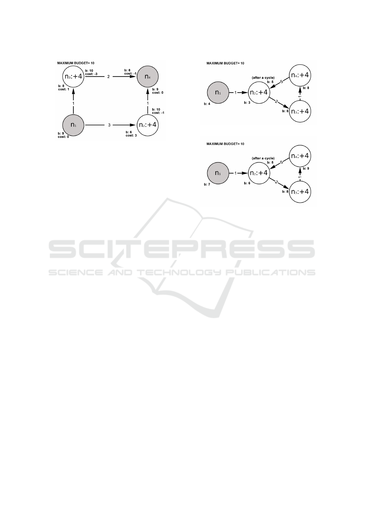
Figure 1: For start node n

, destination node n

and initial

budget 9, the path that minimize the cost (via n

) is not the

same as the path that maximizes the budget (via n

). The

costs are shown on the edges, the gains are shown inside

each node. The maximum budget is 10.

a solution to the problem. Therefore, instead of exit-

ing, we change the algorithm to accept such cycles

and continue as usual. Note that the same cycle can

be beneﬁcial or not depending on the current budget.

The usual operation of BF is to iteratively check

and update the minimum distance for reaching a node.

In our case, we check and update the best budget that

can be achieved by reaching a node (provided there

is sufﬁcient budget to reach that node). It is impor-

tant to note that minimizing the edge costs is not the

same as maximizing the budget, see Figure 1. Also,

due to the maximum budget constraint, the remaining

budget along a path cannot be calculated simply by

subtracting the sum of edge costs from the sum of the

node gains.

The original BF associates each node with a pre-

decessor that corresponds to the previous hop of the

path with the smallest distance so far for that node. A

path can be determined simply by back-tracking the

predecessors from a destination node until the source

node. In our case, we record the entire path. This is

needed because, in the presence of cycles, the knowl-

edge of the predecessor node is not sufﬁcient to re-

construct the path that needs to be followed.

Finally, BF re-computes the distances and node

predecessors |N | − 1 times, where |N | is the num-

ber of nodes in the graph. It is guaranteed that this

sufﬁces to ﬁnd the shortest paths from the destination

node to all nodes. This is not sufﬁcient in our case,

where beneﬁcial cycles may exist and thus paths can

be longer than |N | − 1 hops. For this reason, we run

the algorithm as long as some updates still take place

for some nodes. The algorithm always terminates de-

spite the possibility of having beneﬁcial cycles. Due

to the budget constraint, the same cycle cannot remain

beneﬁcial for ever, see Figure 2. Therefore a cycle can

be performed only a ﬁnite number of times. Note that

(a) Cycle is beneﬁcial.

(b) Cycle is not beneﬁcial.

Figure 2: The same cycle (n

, n

) can be beneﬁcial

(a) or non-beneﬁcial (b), depending on the current budget.

The costs are shown on the edges, the gains are shown in-

side each node. In both cases, the maximum budget is 10.

if there are no beneﬁcial cycles, the algorithm works

like the original version and ﬁnds the optimal path.

4.4 Complexity

The time complexity of MaxBudgetPaths() depends

on the number of the nodes and the number of the

edges in the graph, but also on the number of bene-

ﬁcial cycles and the number of the nodes involved in

them. More concretely, assuming K beneﬁcial cycles

(including any iterations of the same cycle) and an av-

erage of M nodes in each cycle, the time complexity

is O((|N | + K × M) × |E|), where |N | and |E| is the

total number of nodes and the total number of edges

in the graph, respectively. In case no beneﬁcial cycles

exist, the time complexity is the same as the Bellman-

Ford algorithm, O(|N | × |E|). So, the overall com-

plexity of the algorithm (the Skeleton() function) is

O(((|N | + K × M) × |E|) × R), where R is the num-

ber of replannings that are made during the trip of the

vehicle.

5 EVALUATION

We have evaluated the proposed algorithm (we will

refer to it as MaxBudget) for different scenarios. This

VEHITS 2019 - 5th International Conference on Vehicle Technology and Intelligent Transport Systems

section describes the system conﬁguration and the

scenarios that are investigated, and presents results

from indicative experiments.

5.1 Reference Algorithms

To put the performance of the proposed algorithm into

perspective, we use several algorithms as a reference.

These are brieﬂy described in the sequel.

As a ﬁrst reference, we use an oracle algorithm

that has a priori knowledge of the actual edge costs

and node gains that will apply each time the vehicle

were to cross an edge or visit a depot node. The al-

gorithm works in three steps. In the ﬁrst step, it ﬁnds

the minimum cost path from each n

∈ V to each de-

pot node n

∈ D as well as the minimum cost path

from each depot node n

∈ D to each n

∈ V , based

on the actual (known) edge costs. Then, for each de-

pot node n

, it constructs “out” and “in” node clus-

ters. Node n

∈ V belongs to the out cluster of n

if it can be reached from n

with the smallest cost

compared to any other depot node. Node n

∈ V be-

longs to the in cluster of n

if the cost for reaching

is the smallest among all other depot nodes. In

the second step, the algorithm visits as many nodes

of interest it can based on the current budget, before

returning to a depot node to gain some energy (this

is done based on the adapted Bellman-Ford code dis-

cussed earlier). This is repeated, until it is not pos-

sible to visit some of the remaining nodes of interest

and then return to some depot node. Finally, in a third

step, the algorithm tries to visit as many nodes as pos-

sible with the remaining budget (without returning to

a depot node). This is done by running the Held-Karp

algorithm (Held and Karp, 1962), which is an exact

solution to the TSP. Initially, the algorithm is run for

all remaining nodes of interest, let m. If no solution

is found for m, the algorithm is run for m − 1, and if

no solution is found, then it is run for m − 2 etc. If a

solution is found for m ≥ 2, the path returned by the

Held-Karp algorithm is adopted. For m = 1, the algo-

rithm simply picks the cheapest path to any node of

interest, and marks the node as visited if the budget

sufﬁces to reach that node.

We also consider a simpler variant of the above al-

gorithm, which uses static/ﬁxed edge costs and depot

node gains, equal to the mean of the random distribu-

tions, c

mean

and g

mean

. We refer to this as TS-static

since it essentially solves the standard TSP, while tak-

ing into account the energy budget of the vehicle.

As yet another reference, we use an ant colony

optimization (ACO) technique (Jones, 2005). This

is a probabilistic approach for solving path ﬁnding

problems, and has been used expensively in previous

works that study vehicle routing problems and travel-

ing salesman problems. More speciﬁcally, a number

n of ants are generated for m generations and each ant

has a speciﬁc budget. Each ant follows at ﬁrst a ran-

domly chosen route. In our case the ants leave the

pheromone trail of their path if they visit all of the

nodes of interest or their budget is exhausted but they

have achieved the best coverage. The pheromone trail

increases the probability of an ant of a future gener-

ation to choose that speciﬁc path. When an ant stops

traveling, either because it has exhausted its budget or

because it has visited all of the nodes of interest, it

submits its coverage. The algorithm returns the path

that achieves the maximum coverage. Note that ACO

basically solves the same problem as TS-static, using

an approximation heuristic. Several other algorithms

have been proposed for different variants of the VRP,

which could also be adapted to tackle the problem

we study here in order to serve as additional refer-

ences to assess the performance of the proposed algo-

rithm. Such a comprehensive comparison is beyond

the scope of this paper.

Finally, we experiment with a simpler version of

MaxBudget, which performs the path planning step in

normal mode only. As a consequence, the estimates

for the edge costs and depot node gains are always the

mean values of the respective distributions. If no fea-

sible path is found, the algorithm terminates, instead

of switching to the optimistic planning mode.

5.2 Setup and Key Parameters

The topology of the graph used in our experiments is

a 10 × 10 grid, for a total of 100 nodes. Each node is

connected to its horizontal and vertical neighbors via

edges in both directions. The diameter d of the graph

is 18 hops. The grid topology is quite representative

for a terrain where the vehicle can move with a lot of

freedom practically in any direction.

We set the depot nodes to 2% of the total number

of nodes (there are 2 depot nodes). The depot nodes

are chosen randomly, and remain the same throughout

all experiments, at the positions (2, 5) and (8, 6) in the

grid. In all experiments, the vehicle starts its journey

from the node at the bottom-left corner of the grid (at

the position (0, 0). Figure 3 illustrates the setup.

We perform experiments for different sets of

nodes V

⊂ N that need to be visited by the vehi-

cle, where x =

|N |

. We consider four different cases:

x = 5%, 10%, 20% and 30%. For each V

case, we test

the algorithms on three concrete sets, V

, 1 ≤ k ≤ 3.

These are constructed in a random way, however we

make sure that V

⊂ V

in order to

have continuity across the different experiments.

Dynamic Vehicle Routing under Uncertain Travel Costs and Refueling Opportunities

Figure 3: Graph topology used in the experiments. The two

depot nodes are green. The start node is light blue.

With no loss of generality, we set the maximum

budget limit B

max

= 1000. We also set the initial bud-

get of the vehicle b = B

max

= 1000.

For the gain of depot nodes, we adopt a sym-

metrical double-truncated normal distribution with

mean

× B

max

. The rationale behind this choice

is that when the vehicle reaches a depot node with

marginally exhausted budget, on average we want it

to be able to restore its budget to a signiﬁcant degree

(75% of B

max

). The lower and upper bounds are set to

min

= g

mean

−

mean

and g

max

= g

mean

, respec-

tively. In all experiments, we use the same random

distribution for all depot nodes..

The edge costs also follow such a random distribu-

tion with c

min

= c

mean

−

mean

and c

max

= c

mean

In each experiment all edges follow the same cost dis-

tribution, but this varies across experiments. More

speciﬁcally, we let c

mean

max

, where a is the av-

erage number of hops that can be performed by the

vehicle with a maximum initial budget, to which we

refer as the autonomy of the vehicle. We investigate

different degrees of autonomy, set as a function of

the graph diameter: high autonomy d, medium-high

× d, medium-low

× d and low

× d. Higher au-

tonomy enables the vehicle to travel further and visit

a larger number of nodes before visiting a depot node

to regain some energy.

For each of the above autonomy degrees, we pro-

duce 100 different edge cost and node gain scenarios.

The values for the cost of each edge and the gain of

each depot node are produced ofﬂine, and are stored

in a ﬁle from where they are retrieved at runtime.

Note that the cost of an edge changes each time the

edge is crossed; in the scenario ﬁle, 50 different val-

ues are stored for each edge, which are retrieved in a

round-robin fashion each time the vehicle crosses that

particular edge. The same applies to the gain for the

depot nodes. The edge costs and node gains of a sce-

nario are a priori known only to the oracle algorithm.

5.3 Results

For each conﬁguration (combination of V

and a) we

perform different 300 runs (100 scenarios for each

, V

). We report the average coverage for

each algorithm. In order for the ant-colony optimiza-

tion method (ACO) to produce good results, in each

run we use 10 ants and 200 generations of ants. For

the thresholds used in the Check() function of the

MaxBudget algorithm, we set T hreshold

norm

= 10%

and T hreshold

opt

= 4%. These values have been es-

tablished via separate experiments, not reported here

for brevity. Figure 4 shows the results.

It can be seen that MaxBudget consistently

outperforms TS-static. The difference is larger

for mid-range autonomy degrees, in particular for

medium-low where the overall average improvement

is roughly 35% and 44% over V

, V

, and be-

comes smaller for high but also for low autonomy.

This can be explained as follows. On the one hand,

when the autonomy is high, non-optimal decisions

are more tolerable because the vehicle can perform

a larger number of hops without refueling at a de-

pot node. On the other hand, when the autonomy is

low, it becomes much harder to ﬁnd feasible paths,

so the planning decisions of MaxBudget are not good

enough to achieve a high coverage. For the mid-range

autonomy degrees, MaxBudget achieves increasingly

better coverage than TS-static as the number of target

nodes increases. This is because MaxBudget plans

“ahead”, not only to visit the next node of interest,

but also to keep the available energy budget of the ve-

hicle as high as possible when the target is reached,

so that this can be exploited for the next visit. Note

that ACO always performs worse than TS-static. This

is expected as ACO is an approximation of TS-static.

MaxBudget performs close to the oracle for high

and medium-high autonomy. But it cannot match the

oracle for lower degrees of autonomy, where the cov-

erage of MaxBudget drops on average to about 87%

and 67% to that of the oracle, for medium-low and

low autonomy, respectively. Notably, even the oracle

cannot achieve full coverage when the autonomy is

low, in which case it is impossible to visit all nodes of

interest. This also explains why the performance gap

between MaxBudget and TS-static shrinks abruptly in

all low autonomy scenarios, as discussed above.

The simpler version of MaxBudget performs very

close to the full-ﬂedged version of the algorithm. The

fallback to optimistic planning only brings a small

beneﬁt for lower degrees of autonomy, 2.5% on av-

erage for medium-low, and 3.1% for low. In these

cases, optimism occasionally pays-off, allowing the

vehicle to explore paths that would otherwise be re-

VEHITS 2019 - 5th International Conference on Vehicle Technology and Intelligent Transport Systems

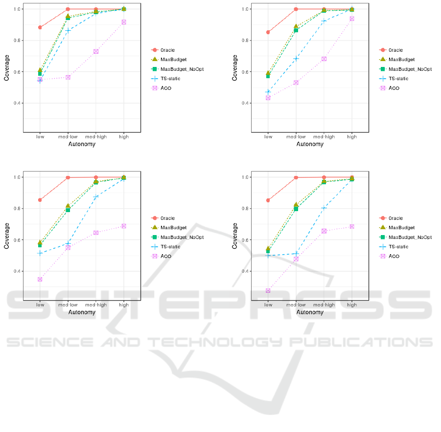
(a) 5 target nodes (V

) (b) 10 target nodes (V

)

) (d) 30 target nodes (V

)

Figure 4: Coverage as a function of the number of nodes to visit and the autonomy of the vehicle.

jected, leading to a few more target node visits. When

the autonomy is relatively high, optimistic planning

does not seem to have any impact.

6 CONCLUSION

We have formulated a variant of the vehicle routing

problem, where both the travel cost and the energy

gain opportunities are stochastic. This is different

than other VRP variants that have been studied in the

literature. Also, we have proposed a heuristic algo-

rithm that can be used to guide an autonomous vehi-

cle in order to visit the nodes of interest; of course, the

same algorithm can be used as a guidance tool for a

human operator. The algorithm is designed for a gen-

eral system model, and can be applied in different ap-

plication scenarios. We have compared our algorithm

with other algorithms, showing that it achieves good

results, especially for system conﬁgurations where it

is indeed feasible to visit all nodes of interest.

In the future, we wish to investigate different vari-

ants of the proposed algorithm in order to improve the

coverage but also to reduce the runtime complexity

(time wise and memory wise). The latter is important

in case it is desirable to run the algorithm directly on

the UV, which will typically have an embedded com-

puting platform with limited memory and processing

capacity. Furthermore, we wish to experiment with

different graph topologies in combination with more

informed values for the edge costs, the node gains and

the budget constraint, based on concrete application

scenarios. It is also interesting to consider how differ-

ent existing algorithms could be adapted to tackle the

variant of the VRP we study in this paper, and to see

how well they perform compared to our algorithm.

ACKNOWLEDGMENTS

This research has been co–ﬁnanced by the Euro-

pean Union and Greek national funds through the

Operational Program Competitiveness, Entrepreneur-

ship and Innovation, under the call RESEARCH -

Dynamic Vehicle Routing under Uncertain Travel Costs and Refueling Opportunities

CREATE - INNOVATE, project PV-Auto-Scout, code

T1EDK-02435.

REFERENCES

Alonso, F., Alvarez, M. J., and Beasley, J. E. (2008). A

tabu search algorithm for the periodic vehicle routing

problem with multiple vehicle trips and accessibility

restrictions. Journal of the Operational Research So-

ciety, 59(7):963–976.

Angelelli, E. and Speranza, M. G. (2002). The periodic ve-

hicle routing problem with intermediate facilities. Eu-

ropean journal of Operational research, 137(2):233–

247.

Artmeier, A., Haselmayr, J., Leucker, M., and Sachen-

bacher, M. (2010). The optimal routing problem in

the context of battery-powered electric vehicles. In

CPAIOR Workshop on Constraint Reasoning and Op-

timization for Computational Sustainability (CROCS).

Bellman, R. (1958). On a routing problem. Quarterly of

applied mathematics, 16(1):87–90.

Bent, R. W. and Van Hentenryck, P. (2004). Scenario-

based planning for partially dynamic vehicle rout-

ing with stochastic customers. Operations Research,

52(6):977–987.

Bertsimas, D. J. (1992). A vehicle routing problem with

stochastic demand. Operations Research, 40(3):574–

585.

Cordeau, J.-F., Gendreau, M., and Laporte, G. (1997). A

tabu search heuristic for periodic and multi-depot ve-

hicle routing problems. Networks: An International

Journal, 30(2):105–119.

Ehmke, J. F., Campbell, A. M., and Urban, T. L. (2015).

Ensuring service levels in routing problems with time

windows and stochastic travel times. European Jour-

nal of Operational Research, 240(2):539–550.

Erera, A. L., Morales, J. C., and Savelsbergh, M. (2010).

The vehicle routing problem with stochastic demand

and duration constraints. Transportation Science,

44(4):474–492.

Escobar, J. W., Linfati, R., Toth, P., and Baldoquin, M. G.

(2014). A hybrid granular tabu search algorithm for

the multi-depot vehicle routing problem. Journal of

heuristics, 20(5):483–509.

Ford Jr, L. R. (1956). Network ﬂow theory. Technical re-

port, Rand Corp Santa Monica Ca.

Gaudioso, M. and Paletta, G. (1992). A heuristic for the

periodic vehicle routing problem. Transportation Sci-

ence, 26(2):86–92.

Gendreau, M., Laporte, G., and S

eguin, R. (1995). An

exact algorithm for the vehicle routing problem with

stochastic demands and customers. Transportation

science, 29(2):143–155.

Gendreau, M., Laporte, G., and S

eguin, R. (1996). A tabu

search heuristic for the vehicle routing problem with

stochastic demands and customers. Operations Re-

search, 44(3):469–477.

Held, M. and Karp, R. M. (1962). A dynamic program-

ming approach to sequencing problems. Journal of

the Society for Industrial and Applied Mathematics,

10(1):196–210.

Jones, K. O. (2005). Ant colony optimization, by marco

dorgio and thomas st

utzle, a bradford book, the mit

press, 2004, xiii+ 305 pp. with index, isbn: 0-262-

04219-3, 475 references at the end.(hardback£ 25.95)-

. Robotica, 23(6):815–815.

Juan, A., Faulin, J., Grasman, S., Riera, D., Marull, J., and

Mendez, C. (2011). Using safety stocks and simula-

tion to solve the vehicle routing problem with stochas-

tic demands. Transportation Research Part C: Emerg-

ing Technologies, 19(5):751–765.

Kenyon, A. S. and Morton, D. P. (2003). Stochastic vehi-

cle routing with random travel times. Transportation

Science, 37(1):69–82.

Laporte, G., Louveaux, F., and Mercure, H. (1992). The

vehicle routing problem with stochastic travel times.

Transportation science, 26(3):161–170.

Laporte, G., Louveaux, F. V., and Van Hamme, L. (2002).

An integer l-shaped algorithm for the capacitated ve-

hicle routing problem with stochastic demands. Oper-

ations Research, 50(3):415–423.

Las Fargeas, J., Hyun, B., Kabamba, P., and Girard, A.

(2012). Persistent visitation with fuel constraints.

Procedia-Social and Behavioral Sciences, 54:1037–

1046.

Marinaki, M. and Marinakis, Y. (2016). A glowworm

swarm optimization algorithm for the vehicle rout-

ing problem with stochastic demands. Expert Systems

with Applications, 46:145–163.

Marinakis, Y., Iordanidou, G.-R., and Marinaki, M. (2013).

Particle swarm optimization for the vehicle routing

problem with stochastic demands. Applied Soft Com-

puting, 13(4):1693–1704.

Mendoza, J. E., Rousseau, L.-M., and Villegas, J. G. (2016).

A hybrid metaheuristic for the vehicle routing prob-

lem with stochastic demand and duration constraints.

Journal of Heuristics, 22(4):539–566.

Mersheeva, V. (2015). UAV Routing Problem for Area Mon-

itoring in a Disaster Situation. PhD thesis.

Miranda, D. M. and Conceic¸

ao, S. V. (2016). The vehicle

routing problem with hard time windows and stochas-

tic travel and service time. Expert Systems with Appli-

cations, 64:104–116.

Rahimi-Vahed, A., Crainic, T. G., Gendreau, M., and Rei,

W. (2013). A path relinking algorithm for a multi-

depot periodic vehicle routing problem. Journal of

heuristics, 19(3):497–524.

Rei, W., Gendreau, M., and Soriano, P. (2010). A hy-

brid monte carlo local branching algorithm for the sin-

gle vehicle routing problem with stochastic demands.

Transportation Science, 44(1):136–146.

Sachenbacher, M., Leucker, M., Artmeier, A., and Hasel-

mayr, J. (2011). Efﬁcient energy-optimal routing for

electric vehicles. In AAAI, pages 1402–1407.

Secomandi, N. (2001). A rollout policy for the vehicle rout-

ing problem with stochastic demands. Operations Re-

search, 49(5):796–802.

VEHITS 2019 - 5th International Conference on Vehicle Technology and Intelligent Transport Systems

Tas¸, D., Dellaert, N., Van Woensel, T., and De Kok, T.

(2013). Vehicle routing problem with stochastic travel

times including soft time windows and service costs.

Computers & Operations Research, 40(1):214–224.

Tas¸, D., Gendreau, M., Dellaert, N., Van Woensel, T., and

De Kok, A. (2014). Vehicle routing with soft time

windows and stochastic travel times: A column gen-

eration and branch-and-price solution approach. Eu-

ropean Journal of Operational Research, 236(3):789–

799.

Van Woensel, T., Kerbache, L., Peremans, H., and Van-

daele, N. (2003). A vehicle routing problem with

stochastic travel times. In Fourth Aegean Interna-

tional Conference on Analysis of Manufacturing Sys-

tems location, Samos, Greece.

Vidal, T., Crainic, T. G., Gendreau, M., Lahrichi, N., and

Rei, W. (2012). A hybrid genetic algorithm for multi-

depot and periodic vehicle routing problems. Opera-

tions Research, 60(3):611–624.

Dynamic Vehicle Routing under Uncertain Travel Costs and Refueling Opportunities