A General Framework to Identify Software Components
from Execution Data
Cong Liu
1
, Boudewijn F. van Dongen
1
, Nour Assy
1
and Wil M.P. van der Aalst
2,1
1
Eindhoven University of Technology, 5600MB Eindhoven, The Netherlands
2
RWTH Aachen University, 52056 Aachen, Germany
Keywords:
Component Identification, Software Execution Data, Community Detection, Empirical Evaluation.
Abstract:
Restructuring an object-oriented software system into a component-based one allows for a better understanding
of the software system and facilitates its future maintenance. A component-based architecture structures a
software system in terms of components and interactions where each component refers to a set of classes. In
reverse engineering, identifying components is crucial and challenging for recovering the component-based
architecture. In this paper, we propose a general framework to facilitate the identification of components
from software execution data. This framework is instantiated for various community detection algorithms,
e.g., the Newman’s spectral algorithm, Louvain algorithm, and smart local moving algorithm. The proposed
framework has been implemented in the open source (Pro)cess (M)ining toolkit ProM. Using a set of software
execution data containing around 1.000.000 method calls generated from four real-life software systems, we
evaluated the quality of components identified by different community detection algorithms. The empirical
evaluation results demonstrate that our approach can identify components with high quality, and the identified
components can be further used to facilitate future software architecture recovery tasks.
1 INTRODUCTION
The maintenance and evolution of software systems
have become a research focus in software engineer-
ing community (Mancoridis et al., 1999). Architec-
tures of these systems can be used as guidance to
help understand and facilitate the future maintenance
(Liu et al., 2018d). However, complete and up-to-date
software architecture descriptions rarely exist (Lind-
vall and Muthig, 2008). Software architectures that
normally include components and interactions can
be reconstructed from low-level data, such as source
code, and execution data.
During the execution of software systems, tremen-
dous amounts of execution data can be recorded. By
exploiting these data, one can reconstruct a software
architecture. To this end, we need to identify com-
ponents from the execution data. For object-oriented
software systems, a component is extracted as a set of
classes that provide a number of functions for other
components. In this paper, we propose a general
framework to identify components from software exe-
cution data by applying various community detection
algorithms. Community detection is one of the most
useful techniques for complex networks analysis with
an aim to identify communities. A software system
can be viewed as a complex network of classes, in
which the component identification problem can be
naturally regarded as the community detection prob-
lem with modularity maximization.
More concretely, we first construct a class interac-
tion graph by exploiting the software execution data
that provides rich information on how classes interact
with each other. Then, different community detec-
tion algorithms are applied to partition the class in-
teraction graph into a set of sub-graphs. Classes that
are grouped in the same sub-graph form a component.
Next, a set of quality criteria are defined to evaluate
the quality of the identified components from differ-
ent perspectives. Our framework definition is generic
and can be instantiated and extended to support vari-
ous community detection algorithms. To validate the
proposed approach, we developed two plug-ins in the
ProM toolkit
1
, which support both the identification
and the evaluation process.
The main contributions of this paper include:
• a general framework to support the identification
and quality evaluation of components from soft-
ware execution data and its instantiation by five
community detection algorithms. Different from
1
http://www.promtools.org/
234
Liu, C., van Dongen, B., Assy, N. and van der Aalst, W.
A General Framework to Identify Software Components from Execution Data.
DOI: 10.5220/0007655902340241
In Proceedings of the 14th International Conference on Evaluation of Novel Approaches to Software Engineering (ENASE 2019), pages 234-241
ISBN: 978-989-758-375-9
Copyright
c
 2019 by SCITEPRESS – Science and Technology Publications, Lda. All rights reserved

existing graph partitioning-based algorithms, our
approach does not require users to specify the
number of clusters in advance; and
• two plug-ins in the ProM toolkit. This allows
other researchers reproducing our experiments
and comparing their approaches.
Section 2 presents some related work. Section 3
defines preliminaries. Section 4 presents the main ap-
proach. Section 5 introduces the tool support. In Sec-
tion 6, we present the experimental evaluation. Fi-
nally, Section 7 concludes the paper.
2 RELATED WORK
Generally speaking, the identification of components
can be achieved by clustering classes. Table 1 sum-
marizes some typical component identification ap-
proaches for object-oriented software systems by con-
sidering the required type of input (i.e., source code,
development documents, execution data), the type of
identification techniques (e.g., graph clustering/parti-
tion, genetic algorithm, etc.), the parameter settings,
and tool support availability. Note that 3/7 means
that the tool is introduced in the paper but is not avail-
able online or does not work any more.
According to Table 1, these approaches are clas-
sified into three categories based on their required in-
put artifacts: (1) development documents-based ap-
proaches that take the sequence diagram, class dia-
gram and use case diagram as input; (2) source code-
based approaches that take the source code as input
and consider structural connections among classes;
and (3) execution data-based approaches that take
software execution data as input. The output of these
approaches are component configurations, i.e., how
classes are grouped to form components. Our work
fits into the third category.
Because software development documents are
typical either incomplete or out-of-date, the appli-
cability of the development documents-based ap-
proaches is quite limited. For components, the idea is
to group together classes that contribute to the same
function. Source code-based approaches use the de-
pendencies among classes that are extracted from the
source code by static analysis techniques. However,
classes in the source code may have in some cases a
wider scope than the functional scope. In addition,
they are not applicable anymore if the source code
is not available (e.g., in case of legacy software sys-
tems). Another way to determine which class con-
tributes to which function (component) is to execute
the software system with individual functions. The
execution data-based approaches help limit the anal-
ysis of dependency only to the space covered by the
application execution. However, existing execution
data-based approaches suffer from the following lim-
itations that may restrict the applicability:
• Requirement for User Input Parameters. Ex-
isting approaches require users to specify a group
of parameters (e.g., the number/size of compo-
nents) as input. However, a reasonable parameter
setting is very difficult for users that are not fa-
miliar with the approach. If parameters are not set
properly, the underlying approaches may perform
badly.
• Lack of a Clearly Defined Systematic Method-
ology. A systematic methodology defines clearly
the required input, the techniques, the resulted
output and the evaluation criteria of the approach
to solve a general research challenge. Existing
execution data-based approaches do not explicitly
define such a complete methodology. This limits
the applicability and extensibility of existing ap-
proaches in the large.
• Lack of Tool Support. The usability of an ap-
proach heavily relies on its tool availability. Exist-
ing dynamic component identification approaches
do not provide usable tools that implement their
techniques. This unavailability prohibits other re-
searchers to reproduce the experiment and com-
pare their approaches.
3 PRELIMINARIES
Let U
M
be the method call universe, U
N
be the
method universe, U
C
be the universe of classes, U
O
be the object universe where objects are instances of
classes. To relate these universes, we introduce the
following notations: For any m ∈ U
M
,
b
m ∈ U
N
is the
method of which m is an instance. For any o ∈ U
O
,
b
o ∈ U
C
is the class of o.
A method call is the basic unit of software execu-
tion data (Liu et al., 2016; Liu et al., 2018d; Liu et al.,
2018a; Liu et al., 2018c; Liu et al., 2018b; Leemans
and Liu, 2017; Qi et al., 2018). The method call and
its attributes are defined as follows:
Definition 1. (Method Call, Attribute) For any m ∈
U
M
, the following standard attributes are defined:
• η : U
M
→ U
O
is a mapping from method calls to
objects such that for each method call m ∈ U
M
,
η(m) is the object containing the instance of the
method
b
m.
• c : U
M
→ U
M
∪ {⊥} is the calling relation among
method calls. For any m
i
, m
j
∈ U
M
, c(m
i
) = m
j
A General Framework to Identify Software Components from Execution Data
235

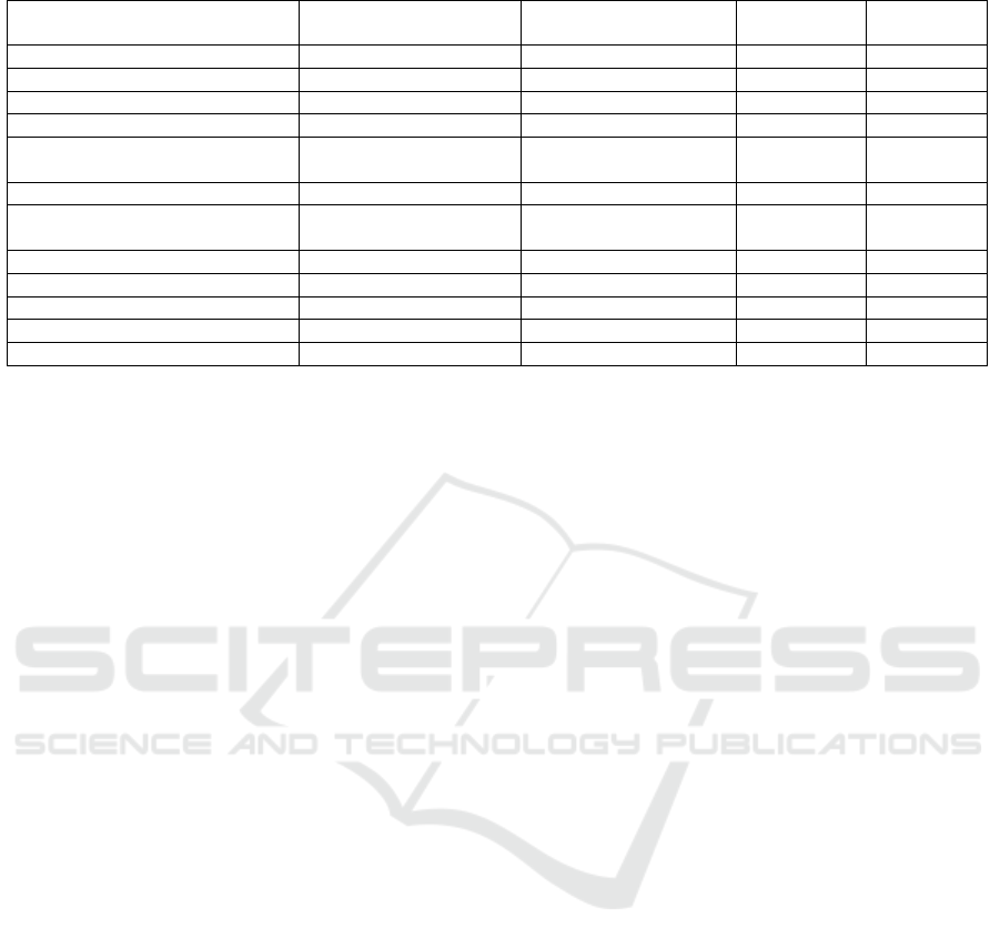
Table 1: Summary of Existing Component Identification Approaches.
Reference Required Input Artifacts Techniques
Parameter
Requirement
Tool
Availability
(Lee et al., 2001) development documents graph clustering 3 7
(Kim and Chang, 2004) development documents use case clustering 3 3/7
(Hasheminejad and Jalili, 2015) development documents evolutionary algorithm 3 7
(Washizaki and Fukazawa, 2005) source code class relation clustering 3 3/7
(Kebir et al., 2012) source code
hierarchical clustering
genetic algorithm
3 7
(Cui and Chae, 2011) source code hierarchical clustering 3 3/7
(Luo et al., 2004) source code
graph clustering
graph iterative analysis
3 7
(Chiricota et al., 2003) source code graph clustering 3 7
(Mancoridis et al., 1999) source code graph partition 3 3/7
(Qin et al., 2009) execution data hyper-graph clustering 3 7
(Allier et al., 2009) execution data concept lattices 3 7
(Allier et al., 2010) execution data genetic algorithm 3 7
means that m
i
is called by m
j
, and we name m
i
as
the callee and m
j
as the caller. For m ∈ U
M
, if
c(m) = ⊥, then
b
m is a main method.
Definition 2. (Software Execution Data) SD ⊆ U
M
is the software execution data.
According to Definition 2, the software execution
data are defined as a finite set of method calls.
4 COMPONENT
IDENTIFICATION
The input of our approach is software execution data,
which can be obtained by instrumenting and monitor-
ing software execution. In Section 4.1, we first give
an overview of the identification framework. Then,
we present the instantiation of the framework with de-
tails in Sections 4.2-4.4.
4.1 Approach Overview
An approach overview is described in the following:
• Class Interaction Graph Construction. Starting
from the software execution data, we construct a
class interaction graph (CIG) where a node rep-
resents a class and an edge represents a calling
relation among the two classes.
• Component Identification. By taking the con-
structed CIG as input, we partition it into a set
of sub-graphs using existing community detection
algorithms. Classes that are grouped in the same
sub-graph form components.
• Quality Evaluation of the Identified Compo-
nents. After identifying a set of components, we
evaluate the quality of the identified components
against the original CIG.
4.2 Class Interaction Graph
Construction
Given the software execution data, we first construct
the CIG according to the following definition.
Definition 3. (Class Interaction Graph) Let SD be
the execution data of a piece of software. G = (V,E)
is defined as the Class Interaction Graph (CIG) of SD
such that:
• V ={v ∈U
C
|∃m∈SD :
[
η(m)=v ∨
\
η(c(m))=v};
• E = {(v
i
, v
j
) ∈ V × V|∃m ∈ SD :
[
η(m) = v
i
∧
\
η(c(m)) = v
j
}.
According to Definition 3, a CIG contains (1) a set
of classes, i.e. vertices; and (2) a set of calling rela-
tions among them, i.e., edges. Note that the calling re-
lations among classes are obtained from method calls,
e.g., if m
1
calls m
2
we have a calling relation saying
the class of m
1
calls the class of m
2
. Different from
existing software call graphs that are defined on top
of the method calling relation in the source code (Qu
et al., 2015), the CIG id defined on the class calling
relations from the execution data.
4.3 Component Identification
After constructing a CIG, we introduce how to iden-
tify components out of the CIG. Essentially, the com-
ponent identification is a division of the vertices of
CIG into a finite set of non-overlapping groups as de-
fined in the following:
Definition 4. (Component Identification) Let SD be
the software execution data and G = (V, E) be its
CIG. CS ⊆ P (V) is defined as the identified compo-
nent set based on certain approach such that:
•
S
C∈CS
C = V; and
ENASE 2019 - 14th International Conference on Evaluation of Novel Approaches to Software Engineering
236

• ∀C
1
, C
2
∈ CS, we have C
1
∩ C
2
=
/
0, i.e., classes
of different components do not overlap.
Definition 4 gives the general idea of component
identification by explicitly defining the input and out-
put, based on which we can see that the identification
does not allow overlaps among components. Note
that this definition can be instantiated by any graph
clustering or community detection techniques.
In the following, we instantiate the component
identification framework by five state-of-the-art com-
munity detection algorithms: (1) the Newman’s spec-
tral algorithm (Newman, 2006) and its MVM refine-
ment (Schaffter, 2014); (2) Louvain algorithm (Blon-
del et al., 2008) and multi-level refinement (Rotta and
Noack, 2011); and (3) Smart local moving algorithm
(Waltman and Van Eck, 2013).
1) Newman’s spectral algorithm and moving ver-
tex method refinement. Newman’s spectral algorithm
aims to determine whether there exists any natural di-
vision of the vertices in a graph/network into nonover-
lapping groups/modules, where these groups/modules
may be of any size. This is addressed by defining a
quantity called modularity Q to evaluate the division
of a set of vertices into modules. Q is defined as fol-
lows: Q = Fe − EFe where Fe represents fraction of
edges falling within modules and EFe represents ex-
pected fraction of such edges in randomized graphs.
To further improve the quality of group structures
inferred using the Newman’s spectral algorithm, a
refinement technique, called Moving Vertex Method
(MVM) is introduced in (Schaffter, 2014). MVM
works independently on top of the detection results
obtained by the Newman’s spectral algorithm. It tries
to move nodes from one community to another com-
munity and checks the effect of the modification on
Q. The modification that leads to the largest increase
in Q is accepted. For more explanations of the MVM
technique refinement, the reader is referred to (New-
man, 2006) and (Schaffter, 2014).
2) Louvain algorithm and multi-level refinement.
The Louvain algorithm starts with each node in a net-
work belonging to its own community, i.e., each com-
ponent consists of one node only. Then, the algo-
rithm uses the local moving heuristic to obtain an im-
proved community structure. The idea of local mov-
ing heuristic is to repeatedly move individual nodes
from one community to another in such a way that
each node movement results in a modularity increase.
Hence, individual nodes are moved from one commu-
nity to another until no further increase in modularity
can be achieved. At this point, a reduced network
where each node refers to a community in the orig-
inal network is constructed. The Louvain algorithm
proceeds by assigning each node in the reduced net-
work to its own singleton community. Next, the local
moving heuristic is applied to the reduced network in
the same way as was done for the original network.
The algorithm continues until a network is obtained
that cannot be reduced further. An extension of the
Louvain algorithm with multi-level refinement is in-
troduced in (Rotta and Noack, 2011). The refinement
improves solutions found by the Louvain algorithm
in such a way that they become locally optimal with
respect to individual node movements.
3) Smart local moving algorithm. The smart lo-
cal moving (SLM) algorithm starts with each node
in a network being its own community and it iter-
ates over all communities in the present community
structure. For each community, a sub-network is con-
structed which is a copy of the original network that
includes only the nodes belonging to a specific com-
munity of interest. The SLM algorithm then uses the
local moving heuristic to identify communities in the
sub-network. Each node in the sub-network is first
assigned to its own singleton community, and then lo-
cal moving heuristic is applied. After a community
structure has been obtained for each sub-network, the
SLM algorithm constructs a reduced network. In the
reduced network, each node corresponds to a com-
munity in one of the sub-networks. The SLM al-
gorithm then performs an initial assignment of the
nodes to communities in the reduced network in such
a way that nodes corresponding to communities in the
same sub-network are assigned to the same commu-
nity. The previous steps start over again for the re-
duced network until a network is obtained that cannot
be reduced any more.
4.4 Quality Metrics
This section introduces a group of quality metrics to
help evaluate the components identified by different
community detection techniques.
1) Size and Counting.
To give a general overview of the identified com-
ponents, we first introduce the following metrics:
• The number of identified components (NoC) from
the execution data of a software system.
• The average size of identified components (AoC),
i.e., the average number of classes that each com-
ponent involves.
• The ratio of single class components (RSC). RSC
means the number of classes in single class com-
ponents divided by the total number of classes.
• The ratio of largest component (RLC). RLC rep-
resents the number of classes in the largest com-
ponent divided by the total number of classes.
A General Framework to Identify Software Components from Execution Data
237

• The ratio of intermediate components (RIC). RIC
represents the number of classes in the interme-
diate components divided by the total number of
classes. Note that RICs refer to components that
neither contains one class nor be the largest ones.
According to (Cui and Chae, 2011), components
with very large number of classes (high RLC) or very
small number of classes (high RSC) cannot be re-
garded as good components. An ideal distribution is
a normal distribution where quite many components
have reasonable size (high RIC). Hence, we should
try to avoid the case of too many single class compo-
nents as well as a single very large one.
2) Coupling. In component-based software sys-
tems, coupling represents how tightly one compo-
nent interacts with the others. The coupling metric
between two components is defined as the ratio of
the number of edges connecting them to the maximal
number of edges that connect all their vertices.
Let G = (V, E) be a CIG and CS be the identified
components. For any C
1
, C
2
∈ CS, we have:
coupl(C
1
,C
2
) =
|CouEdge|
|C
1
| × |C
2
|
(1)
where CouEdge = E ∩ ((C
1
× C
2
) ∪ (C
2
× C
1
)) rep-
resents the set of edges that connecting components
C
1
and C
2
. Then, the coupling metric of all compo-
nents is defined as follows:
Coupling(CS) =
∑
1≤i<j≤|CS|
coupl(C
i
, C
j
)
|CS| × (|CS| − 1)
(2)
3) Cohesion. In component-based software sys-
tems, cohesion represents how tightly classes in the
same component are associated. The cohesion metric
of a component is defined as the ratio of the number
of its edges to the maximal number of edges that can
connect all its vertices (the number of edges in the
complete graph on the set of vertices).
For any C∈CS, its cohesion metric is defined as:
cohes(C) =
|CohEdge(C)|
|C| × (|C| − 1)
(3)
where CohEdge(C) = E ∩ (C × C) represents the set
of edges that are contained in C. Then, the cohesion
metric of all components is defined as follows:
Cohesion(CS) =
∑
C∈CS
cohes(C)
|CS|
(4)
4) Modularity Quality. The cohesion and cou-
pling metrics measure the quality of the identifica-
tion results from two opposite perspectives. A well-
organized component-based architecture should be
highly cohesive and loosely coupled.
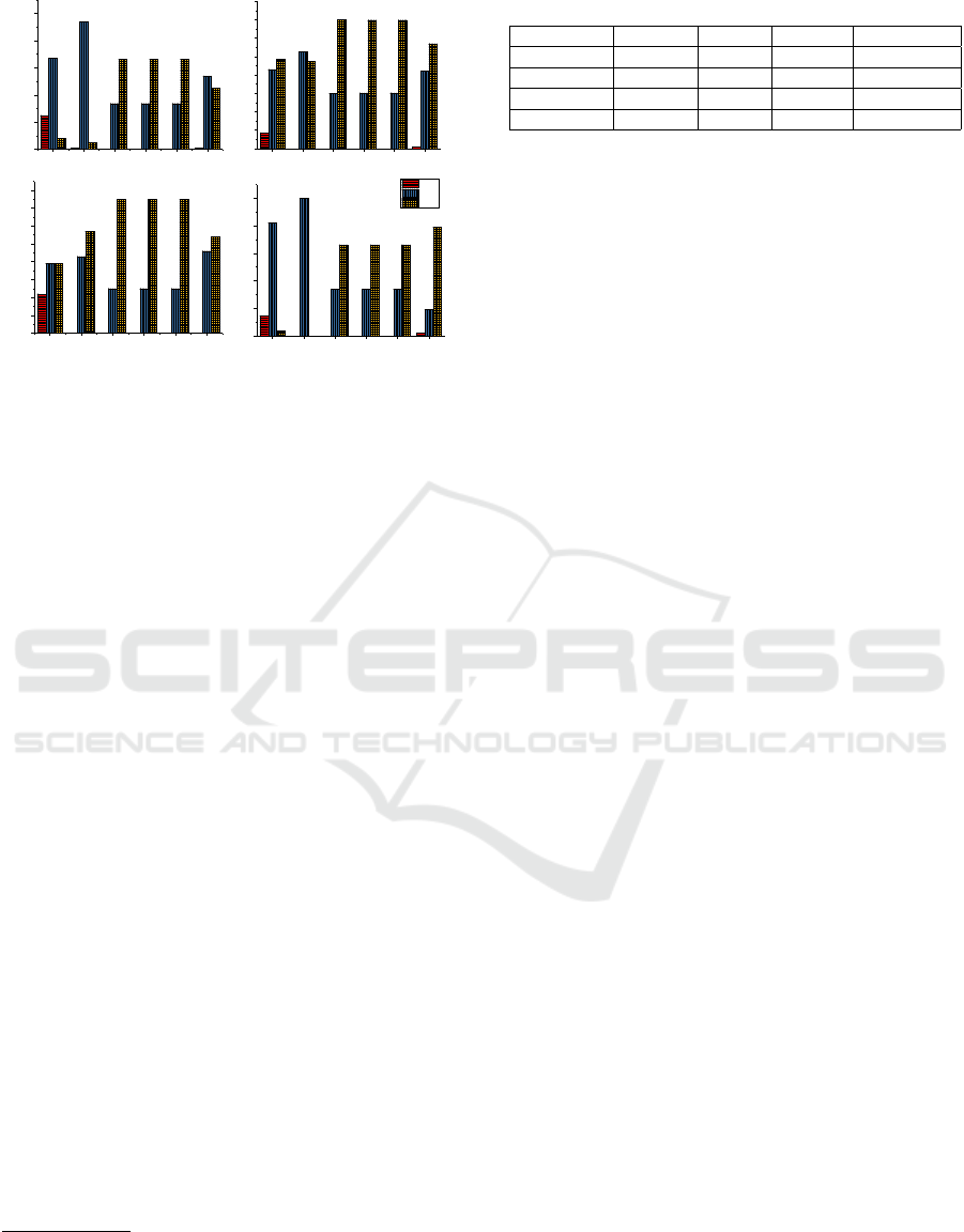
Table 2: Number and Size of Identified Components.
Lexi 0.1.1 JHotDraw 5.1 JUnit 3.7 JGraphx 3.5.1
NoC AoC NoC AoC NoC AoC NoC AoC
NSA 20 3.4 13 7.1 9 5.2 11 5.6
NSA-R 3 22.3 5 18.6 4 10.2 1 62
SLM 5 13.6 6 15.5 5 9.4 5 12.4
LA 5 13.6 6 15.5 5 9.4 5 12.4
LA-R 5 13.6 7 13.3 5 9.4 5 12.4
Base 5 13.6 7 13.3 3 15.6 9 6.9
Modularity Quality (MQ) aims to reward the cre-
ation of highly cohesive components and to penalize
excessive coupling among them. It is formally de-
fined as follows:
MQ(CS) = Cohesion(CS) − Coupling(CS) (5)
MQ lies in the [−1, 1] interval and a higher MQ
value normally means a better architecture quality.
5 IMPLEMENTATION IN PROM
The open-source (Pro)cess (M)ining framework
ProM 6
2
provides a completely plugable environment
for process mining and related topics. It can be ex-
tended by adding plug-ins, and currently, more than
1600 plug-ins are included.
The component identification and quality evalua-
tion approaches have been implemented as two plug-
ins in our ProM 6 package
3
. The first one, called In-
tegrated Component Identification Framework, takes
as input the software execution data, and returns the
component configuration file that describes which
classes belong to which components. Note that this
plugin currently supports all community detection al-
gorithms introduced in Section 4.3. The second plu-
gin, called Quality Measure of Component Identifi-
cation, takes (1) the software execution data and (2)
component configuration as input, and returns the
quality metrics (e.g., size and modularity values) of
the identification component configuration. All ex-
perimental results in the following discussions are
based on these two tools.
6 EXPERIMENTAL EVALUATION
Then, we evaluate our approaches using four open-
source software systems.
2
http://www.promtools.org/
3
https://svn.win.tue.nl/repos/prom/Packages/SoftwareProcessMining/
ENASE 2019 - 14th International Conference on Evaluation of Novel Approaches to Software Engineering
238

0 . 2 5
0 . 0 1
0 0 0
0 . 0 1
0 . 6 7
0 . 9 4
0 . 3 3 8 0 . 3 3 8 0 . 3 3 8
0 . 5 4
0 . 0 8
0 . 0 5
0 . 6 6 2 0 . 6 6 2 0 . 6 6 2
0 . 4 5
N S A N S A - R S L M L A L A - R B a s e l i n e
0 . 0
0 . 2
0 . 4
0 . 6
0 . 8
1 . 0
S i z e
(a) Lexi 0.1.1
0 . 0 8 6
0 0 0 0
0 . 0 1
0 . 4 3
0 . 5 2 6
0 . 3
0 . 3 0 2 0 . 3 0 2
0 . 4 2
0 . 4 8 4
0 . 4 7 4
0 . 7
0 . 6 9 8 0 . 6 9 8
0 . 5 7
N S A N S A - R S L M L A L A - R B a s e l i n e
0 . 0
0 . 1
0 . 2
0 . 3
0 . 4
0 . 5
0 . 6
0 . 7
0 . 8
S i z e
(b) JHotDraw 5.1
0 . 2 2
0 0 0 0 0
0 . 3 9
0 . 4 3
0 . 2 5 0 . 2 5 0 . 2 5
0 . 4 6
0 . 3 9
0 . 5 7
0 . 7 5 0 . 7 5 0 . 7 5
0 . 5 4
N S A N S A - R S L M L A L A - R B a s e l i n e
0 . 0
0 . 1
0 . 2
0 . 3
0 . 4
0 . 5
0 . 6
0 . 7
0 . 8
S i z e
(c) JUnit 3.7
0 . 1 4 5
0 0 0 0
0 . 0 2
0 . 8 2
1
0 . 3 3 8 0 . 3 3 8 0 . 3 3 8
0 . 1 9
0 . 0 3 5
0
0 . 6 6 2 0 . 6 6 2 0 . 6 6 2
0 . 7 9
N S A N S A - R S L M L A L A - R B a s e l i n e
0 . 0
0 . 2
0 . 4
0 . 6
0 . 8
1 . 0
R S C
R L C
R I C
S i z e
(d) JGraphx 3.5.1
Figure 1: Size Comparison.
6.1 Subject Software Systems and
Execution Data
For our experiments, we use the execution data that
are collected from four open-source software systems.
More specifically, Lexi 0.1.1
4
is a Java-based open-
source word processor. Its main function is to cre-
ate documents, edit texts, save files, etc. The format
of exported files are compatible with Microsoft word.
JHotDraw 5.1
5
is a GUI framework for technical and
structured 2D Graphics. Its design relies heavily on
some well-known GoF design patterns. JUnit 3.7
6
is a simple framework to write repeatable tests for
java programs. It is an instance of the xUnit archi-
tecture for unit testing frameworks. JGraphx 3.5.1
7
is an open-source family of libraries that provide fea-
tures aimed at applications that display interactive di-
agrams and graphs.
Note that the execution data of Lexi 0.1.1,
JGraphx 3.5.1, and JHotDraw 5.1 are collected by
monitoring typical execution scenarios of the soft-
ware systems. For example, a typical scenario of the
JHotDraw 5.1 is: launch JHotDraw, draw two rectan-
gles, select and align the two rectangles, color them
as blue, and close JHotDraw. For the JUnit 3.7, we
monitor the execution of the project test suite with
259 independent tests provided in the MapperXML
8
release. Table 3 shows the detailed statistics of the
data execution, including the number of packages/-
classes/methods that are loaded during execution and
the number of method calls analyzed.
4
http://essere.disco.unimib.it/svn/DPB/Lexi%20v0.1.1%20alpha/
5
http://www.inf.fu-berlin.de/lehre/WS99/java/swing/JHotDraw5.1/
6
http://essere.disco.unimib.it/svn/DPB/JUnit%20v3.7/
7
https://jgraph.github.io/mxgraph/
8
http://essere.disco.unimib.it/svn/DPB/MapperXML%20v1.9.7/
Table 3: Statistics of Subject Software Execution Data.
Software #Packages #Classes #Methods #Method Calls
Lexi 0.1.1 5 68 263 20344
JHotDraw 5.1 7 93 549 583423
JUnit 3.7 3 47 213 363948
JGraphx 3.5.1 9 62 695 74842
6.2 Identification Approaches
Five component identification approaches are evalu-
ated with respect to a baseline. The first approach
identifies components by the Newman’s spectral algo-
rithm (denoted as NSA). The second approach iden-
tifies components by Newman’s spectral algorithm
with MVM refinement (denoted as NSA-R). The third
one creates a component based on smart local mov-
ing algorithm (denoted as SLM). The forth approach
identifies components by the Louvain algorithm (de-
noted as LA). Finally, the last one identifies compo-
nents by the Louvain algorithm with multi-level re-
finement (denoted as LA-R).
To evaluate the quality of identified components,
we compare them with a baseline. The packages that
are defined in the source code are assumed as compo-
nents manually classified by software developers in
the design stage, and are used as the baseline in the
following experiments.
6.3 Evaluation Results
In this section, we evaluate the quality of the compo-
nents identified by different approaches as well as the
baseline. More specifically, we first identify compo-
nents for the four software systems using NSA, NSA-
R, SLM, LA and LA-R. Afterwards, the quality of com-
ponents is measured and compared in terms of size
and modularity metrics that are defined in Section
4.4. In addition, the time performance of different
approaches are also compared.
The number of identified components (NoC) and
the average size of components (AoC) for the four
open-source software systems based on NSA, NSA-R,
SLM, LA, LA-R, and the baseline are shown in Table 2.
Note that the AoC value decreases as the NoC value
increases for each software system. This is because
the AoC is computed as the total number of classes
divided by NoC. In general, the NoC/AoC values of
NSA-R, SLM, LA and LA-R are similar with the base-
line while the NoC/AoC value of NSA is much higher
than others, i.e., too much components are identified
by NSA for each software system.
Fig. 1 shows the size metric evaluation results
for Lexi 0.1.1, JHotDraw 5.1, JUnit 3.7 and JGraphx
3.5.1 based on NSA, NSA-R, SLM, LA, LA-R, and the
A General Framework to Identify Software Components from Execution Data
239

0 . 0 5 8
0 . 2 3 8
0 . 2 6 6 0 . 2 6 6 0 . 2 6 6
0 . 1 6
N S A N S A - R S L M L A L A - R B a s e l i n e
0 . 0 0
0 . 0 5
0 . 1 0
0 . 1 5
0 . 2 0
0 . 2 5
0 . 3 0
M o d u l a r i t y
(a) Lexi 0.1.1
0 . 0 5 8
0 . 2 3 8
0 . 2 6 6 0 . 2 6 6 0 . 2 6 6
0 . 1 6
N S A N S A - R S L M L A L A - R B a s e l in e
0 . 0 0
0 . 0 5
0 . 1 0
0 . 1 5
0 . 2 0
0 . 2 5
0 . 3 0
M o d u l a r i t y
(b) JHotDraw 5.1
0 . 0 9
0 . 2 9 2
0 . 3 1 3 0 . 3 1 3 0 . 3 1 3
0 . 1 6 1
N S A N S A - R S L M L A L A - R B a s e l i n e
0 . 0 0
0 . 0 5
0 . 1 0
0 . 1 5
0 . 2 0
0 . 2 5
0 . 3 0
0 . 3 5
M o d u l a r i t y
(c) JUnit 3.7
0 . 0 5 3
0 . 1 2
0 . 2 8 0 . 2 8 0 . 2 8
0 . 2 2
N S A N S A - R S L M L A L A - R B a s e l i n e
0 . 0 0
0 . 0 5
0 . 1 0
0 . 1 5
0 . 2 0
0 . 2 5
0 . 3 0
M o d u l a r i t y
(d) JGraphx 3.5.1
Figure 2: Modularity Comparison.
baseline. Normally, a higher RIC (or low RSC and
RLC) value indicates that the identified components
are more well-organized than those with lower RIC
(or high RSC and RLC) values. Generally speaking,
the RIC values of SLM, LA and LA-R are much higher
than those of NSA and NSA-R as well as the baseline.
As for the SLM, LA and LA-R, they have almost the
same results. This can be explained by the fact that
all these three approaches are based on the local mov-
ing heuristic. Different from this general conclusion,
there are some exceptions. Considering for example
the JGraphx 3.5.1. The RIC value of the baseline is
much higher than those of SLM, LA and LA-R. This
indicates that the package structure of the JGraphx
3.5.1 is better-organized than those of other software.
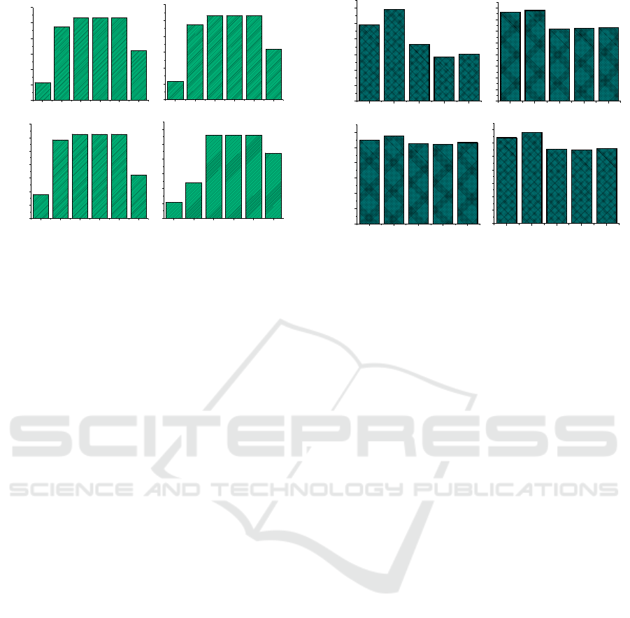
Fig. 2 shows the evaluation results in terms of the
MQ for the four software systems. This metric mea-
sures the quality of the identified components from an
architectural point of view. A higher MQ value nor-
mally indicates that the identified components lead to
a better software architecture quality than those with
lower MQ values. Generally speaking, the MQ values
of SLM, LA and LA-R are much higher than those of
NSA and NSA-R as well as the baseline. In addition,
NSA-R always performs better than NSA for the four
software systems. The rationale behind is that NSA-R
refines the results of NSA with the aim to improve the
overall modularity.
Fig. 3 shows the time performance comparison
results in terms of milliseconds for the four soft-
ware systems. An approach with a lower performance
value indicates that it is more efficient than that with
a higher value. Generally speaking, SLM, LA and LA-
R are more efficient than NSA and NSA-R according
to Fig. 3. As for LA and LA-R, LA is always more
efficient than LA-R because LA-R requires a further
refinement step on top of the results of LA.
2 4 7
2 9 7
1 8 4
1 4 3
1 5 1
N S A N S A - R S L M L A L A - R
0
5 0
1 0 0
1 5 0
2 0 0
2 5 0
3 0 0
E x e c u t i o n T i m e / m s
(a) Lexi 0.1.1
3 8 1 4
3 9 0 0
3 1 0 0
3 1 3 6
3 1 6 9
N S A N S A - R S L M L A L A - R
0
5 0 0
1 0 0 0
1 5 0 0
2 0 0 0
2 5 0 0
3 0 0 0
3 5 0 0
4 0 0 0
E x e c u t i o n T i m e / m s
(b) JHotDraw 5.1
2 7 4 6
2 8 8 3
2 6 3 3
2 6 1 8
2 6 6 8
N S A N S A - R S L M L A L A - R
0
5 0 0
1 0 0 0
1 5 0 0
2 0 0 0
2 5 0 0
3 0 0 0
E x e c u t i o n T i m e / m s
(c) JUnit 3.7
6 4 2
6 7 9
5 5 4
5 5 0
5 5 9
N S A N S A - R S L M L A L A - R
0
1 0 0
2 0 0
3 0 0
4 0 0
5 0 0
6 0 0
7 0 0
E x e c u t i o n T i m e / m s
(d) JGraphx 3.5.1
Figure 3: Time Performance Comparison.
In summary, compared with NSA, NSA-R, SLM
and LA, LA-R can efficiently (from a performance
point of view) identify components with high MQ val-
ues, which can help reconstruct the software architec-
ture with better quality. Based on the experimental
evaluation, we recommend to apply the LA-R to iden-
tify components for architecture recovery from soft-
ware execution data.
7 CONCLUSION
By exploiting tremendous amounts of software exe-
cution data, we can identify a set of components for
a given software system. Our proposed approaches
have been implemented in the ProM toolkit and its
advantage and usability were demonstrated by apply-
ing them to a set of software execution data generated
from four different real-life software systems.
This paper provides a concrete step to reconstruct
the architecture from software execution data by iden-
tifying a set of components. If the execution data
does not cover certain part of the software, our ap-
proach fails to identify interaction between classes. In
this scenario, combination of the static analysis tech-
niques (i.e., source code) and dynamic analysis tech-
niques (i.e., execution data) is desired. Another future
challenge is to discover how components interact with
each other via interfaces as well as reconstructing the
overall software architecture. In addition, we will
conduct an empirical evaluation to compare the qual-
ity of the recovered architectural models using differ-
ent component identification techniques (e.g., (Allier
et al., 2009; Qin et al., 2009)) and interface identifi-
cation techniques (e.g., (Liu et al., 2018a)).
ENASE 2019 - 14th International Conference on Evaluation of Novel Approaches to Software Engineering
240

REFERENCES
Allier, S., Sahraoui, H., Sadou, S., and Vaucher, S.
(2010). Restructuring object-oriented applications
into component-oriented applications by using consis-
tency with execution traces. Component-Based Soft-
ware Engineering, pages 216–231.
Allier, S., Sahraoui, H. A., and Sadou, S. (2009). Identi-
fying components in object-oriented programs using
dynamic analysis and clustering. In Proceedings of
the 2009 Conference of the Center for Advanced Stud-
ies on Collaborative Research, pages 136–148. IBM
Corp.
Blondel, V. D., Guillaume, J.-L., Lambiotte, R., and Lefeb-
vre, E. (2008). Fast unfolding of communities in large
networks. Journal of statistical mechanics: theory
and experiment, 2008(10):P10008.
Chiricota, Y., Jourdan, F., and Melanc¸on, G. (2003). Soft-
ware components capture using graph clustering. In
Program Comprehension, 2003. 11th IEEE Interna-
tional Workshop on, pages 217–226. IEEE.
Cui, J. F. and Chae, H. S. (2011). Applying agglomerative
hierarchical clustering algorithms to component iden-
tification for legacy systems. Information and Soft-
ware technology, 53(6):601–614.
Hasheminejad, S. M. H. and Jalili, S. (2015). Ccic: Cluster-
ing analysis classes to identify software components.
Information and Software Technology, 57:329–351.
Kebir, S., Seriai, A.-D., Chardigny, S., and Chaoui, A.
(2012). Quality-centric approach for software compo-
nent identification from object-oriented code. In Soft-
ware Architecture (WICSA) and European Conference
on Software Architecture (ECSA), 2012 Joint Working
IEEE/IFIP Conference on, pages 181–190. IEEE.
Kim, S. D. and Chang, S. H. (2004). A systematic method
to identify software components. In 11th Asia-Pacific
Software Engineering Conference, 2004., pages 538–
545. IEEE.
Lee, J. K., Jung, S. J., Kim, S. D., Jang, W. H., and Ham,
D. H. (2001). Component identification method with
coupling and cohesion. In Eighth Asia-Pacific Soft-
ware Engineering Conference, 2001. APSEC 2001.,
pages 79–86. IEEE.
Leemans, M. and Liu, C. (2017). Xes software event exten-
sion. XES Working Group, pages 1–11.
Lindvall, M. and Muthig, D. (2008). Bridging the software
architecture gap. Computer, 41(6).
Liu, C., van Dongen, B., Assy, N., and van der Aalst, W.
(2016). Component behavior discovery from software
execution data. In International Conference on Com-
putational Intelligence and Data Mining, pages 1–8.
IEEE.
Liu, C., van Dongen, B., Assy, N., and van der Aalst, W.
(2018a). Component interface identification and be-
havior discovery from software execution data. In
26th International Conference on Program Compre-
hension (ICPC 2018), pages 97–107. ACM.
Liu, C., van Dongen, B., Assy, N., and van der Aalst, W.
(2018b). A framework to support behavioral design
pattern detection from software execution data. In
13th International Conference on Evaluation of Novel
Approaches to Software Engineering, pages 65–76.
Liu, C., van Dongen, B., Assy, N., and van der Aalst, W.
(2018c). A general framework to detect behavioral de-
sign patterns. In International Conference on Software
Engineering (ICSE 2018), pages 234–235. ACM.
Liu, C., van Dongen, B., Assy, N., and van der Aalst, W.
(2018d). Software architectural model discovery from
execution data. In 13th International Conference on
Evaluation of Novel Approaches to Software Engi-
neering, pages 3–10.
Luo, J., Jiang, R., Zhang, L., Mei, H., and Sun, J. (2004).
An experimental study of two graph analysis based
component capture methods for object-oriented sys-
tems. In Software Maintenance, 2004. Proceedings.
20th IEEE International Conference on, pages 390–
398. IEEE.
Mancoridis, S., Mitchell, B. S., Chen, Y., and Gansner,
E. R. (1999). Bunch: A clustering tool for the recov-
ery and maintenance of software system structures.
In Software Maintenance, 1999.(ICSM’99) Proceed-
ings. IEEE International Conference on, pages 50–59.
IEEE.
Newman, M. E. (2006). Modularity and community struc-
ture in networks. Proceedings of the national academy
of sciences, 103(23):8577–8582.
Qi, J., Liu, C., Cappers, B., and van de Wetering, H.
(2018). Visual analysis of parallel interval events. In
20th EG/VGTC Conference on Visualization (EuroVis
2018), pages 1–6.
Qin, S., Yin, B.-B., and Cai, K.-Y. (2009). Mining compo-
nents with software execution data. In International
Conference Software Engineering Research and Prac-
tice., pages 643–649. IEEE.
Qu, Y., Guan, X., Zheng, Q., Liu, T., Wang, L., Hou, Y., and
Yang, Z. (2015). Exploring community structure of
software call graph and its applications in class cohe-
sion measurement. Journal of Systems and Software,
108:193–210.
Rotta, R. and Noack, A. (2011). Multilevel local search
algorithms for modularity clustering. Journal of Ex-
perimental Algorithmics (JEA), 16:2–3.
Schaffter, T. (2014). From genes to organisms: Bioin-
formatics System Models and Software. PhD thesis,
´
Ecole Polytechnique F
´
eD
´
erale de Lausanne.
Waltman, L. and Van Eck, N. J. (2013). A smart local mov-
ing algorithm for large-scale modularity-based com-
munity detection. The European Physical Journal B,
86(11):471.
Washizaki, H. and Fukazawa, Y. (2005). A technique for
automatic component extraction from object-oriented
programs by refactoring. Science of Computer pro-
gramming, 56(1-2):99–116.
A General Framework to Identify Software Components from Execution Data
241