
Flexible IoT Edge Computing System to Solve the Tradeoff of
Optimal Route Search
Tadashi Ogino
School of Information Science, Meisei University, Tokyo, Japan
Keywords: IoT, Edge Computing, Cloud Computing, ITS.
Abstract: In recent times, large-scale cloud computing based Internet of Things (IoT) systems are facing problems
such as an increase in network load, delay in response, and invasion of privacy. To solve these problems,
edge computing technique has been employed in many IoT systems. However, if the cloud function is
excessively migrated to the edge, the collected data cannot be shared between IoT systems, thus, reducing
the system's usefulness. We propose a multi-agent based flexible IoT edge computing architecture to
balance global optimization by a cloud and local optimization by edges and to optimize the role of both the
cloud and the edge servers in a dynamic manner. In this paper, as an application example, we introduce a
route search system based on the proposed edge computing system architecture to demonstrate the
effectiveness of the proposed method.
1 INTRODUCTION
Internet of Things (IoT) systems, a new paradigm in
which many sensors or devices are connected
directly to the Internet to provide various services
without human intervention, have been attracting
attention in recent times (Al-Fuqaha et al., 2015).
IoT applications are adopted in the industrial,
household, as well as social sectors. These
conventional IoT systems are based on cloud-centric
architecture. Therefore, problems such as an
increase in network load delayed feedback response,
and privacy invasion is identified in a large-scale
IoT system (Abdelshkour, 2015).
To solve these problems, the concept of edge
computing (EC) has been introduced to the IoT
architecture (Lopez et al., 2015). EC is effective in
solving communication traffic shortage and delayed
feedback control issues. However, if the cloud
functions are excessively migrated to the edge, the
collected data cannot be shared between IoT systems
and this decreases the system's usefulness (Shiratori
et al., 2017). Moreover, while EC is effective for
local optimization in an edge domain, it is not
effective in realizing global optimization of multiple
domains.
Our previous research (Ogino et al., 2017)
proposed a multi-agent based flexible IoT-EC
architecture to solve these problems of the
conventional EC. The proposed IoT architecture
balances global optimization by a cloud and local
optimization by edges to optimize the roles of the
cloud server and the edge servers dynamically using
multi-agent technology.
In this paper, we apply the proposed
architecture to a traffic control system. We
demonstrate the effectiveness of our proposed
architecture through traffic simulation.
2 BACKGROUND OF THIS
RESEARCH
2.1 Conventional Cloud-Centric Iot
Architecture
Various types of IoT architectures have been
proposed by standards bodies and researchers (Yang
et al., 2011). A couple of architectures are based on
a three-layer IoT architecture, as shown in Figure
1(a). Another type of architecture is the five-layer
IoT architecture that extracts common functions
from the three-layer IoT architecture and adds a
business layer to it. Figure 1 (b) is one example of a
five-layer IoT architecture (Al-Fuqaha et al., 2015).
Ogino, T.
Flexible IoT Edge Computing System to Solve the Tradeoff of Optimal Route Search.
DOI: 10.5220/0007587702150222
In Proceedings of the 4th International Conference on Internet of Things, Big Data and Security (IoTBDS 2019), pages 215-222
ISBN: 978-989-758-369-8
Copyright
c
2019 by SCITEPRESS – Science and Technology Publications, Lda. All rights reserved
215
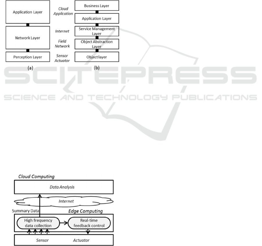
In the five-layered IoT architecture, all the data
is collected and analyzed in the cloud. Furthermore,
all the actuators in the object layer are controlled by
the results in the cloud. This approach has some
demerits (Abdelshkour, 2015). They are as follows.
1) Under a large IoT system containing several
sensors, collecting a large amount of data leads
to communication traffic shortage.
2) The communication convergence on the
Internet and the cloud cause control delay. The
system delay also depends on the frequency of
the data collection.
3) Storing all the data in the cloud causes serious
security issues.
Figure 1: IoT Architecture: a) Three-layer IoT
Architecture; b) Five-layer IoT Architecture.
2.2 IoT Edge Computing
The concept of EC was introduced to the IoT
architecture to solve the problems highlighted in the
previous section (Ren et al., 2017).
EC is a method of performing data processing at
a place near the data origin or control targets. Figure
2 shows the IoT architecture with a three-layer EC
system. In this architecture, data collection, filtering,
and feedback control functions are implemented on
edge servers.
Figure 2: IoT-EC.
2.3 Problems of IoT Edge Computing
IoT-EC architecture is effective in solving network
traffic shortage and delay in feedback control.
However, there are a couple of problems facing IoT-
EC as described below (Shiratori et al., 2017).
Problem-1) Provisioning of IoT functions depends
on the resources and network environment of the
edge servers. We need a method to optimize all IoT
systems by changing the roles of the cloud and the
edge part dynamically according to the resources
and network environment of the edge servers.
Problem-2) If all the IoT functions are placed at
the edge servers, all the IoT systems become the
localized vertical integrated system. This prevents
global optimization based on the collected data. On
the contrary, prioritizing global optimization in
cloud hinders local optimization such as real-time
control in the edge. In other words, when we
introduce EC to the IoT system, we need a
mechanism to balance global optimization in the
cloud and local optimization at the edges of the
network.
3 FLEXIBLE MULTI-AGENT
BASED IoT EDGE COMPUTING
There have been consistent research efforts
(Kitagami et al., 2016; Suganuma et al., 2016;
Shiratori et al., 2017) that aim to solve the problems
of IoT-EC described in the previous section. Based
on the concept presented in the previous research,
we proposed a flexible IoT-EC architecture (Ogino
et al., 2017) to solve Problem-2 of IoT-EC. In this
paper, after discussing the basic concept of flexible
IoT-EC architecture, we discussed how to apply the
proposed architecture to a traffic control system.
3.1 Basic Concept
Herein, we discuss how total balancing mechanisms
between cloud and edges work in the proposed
architecture.
The balancing optimization functions are divided
into cloud-side and the edge-side. Each optimization
subtask can only optimize its side because it does
not have enough information of another side. There
is often a tradeoff in the relationship between the
cloud and the edges especially for actual
applications. By simply improving the performance
IoTBDS 2019 - 4th International Conference on Internet of Things, Big Data and Security
216
of one side, the performance of the other side may
decrease.
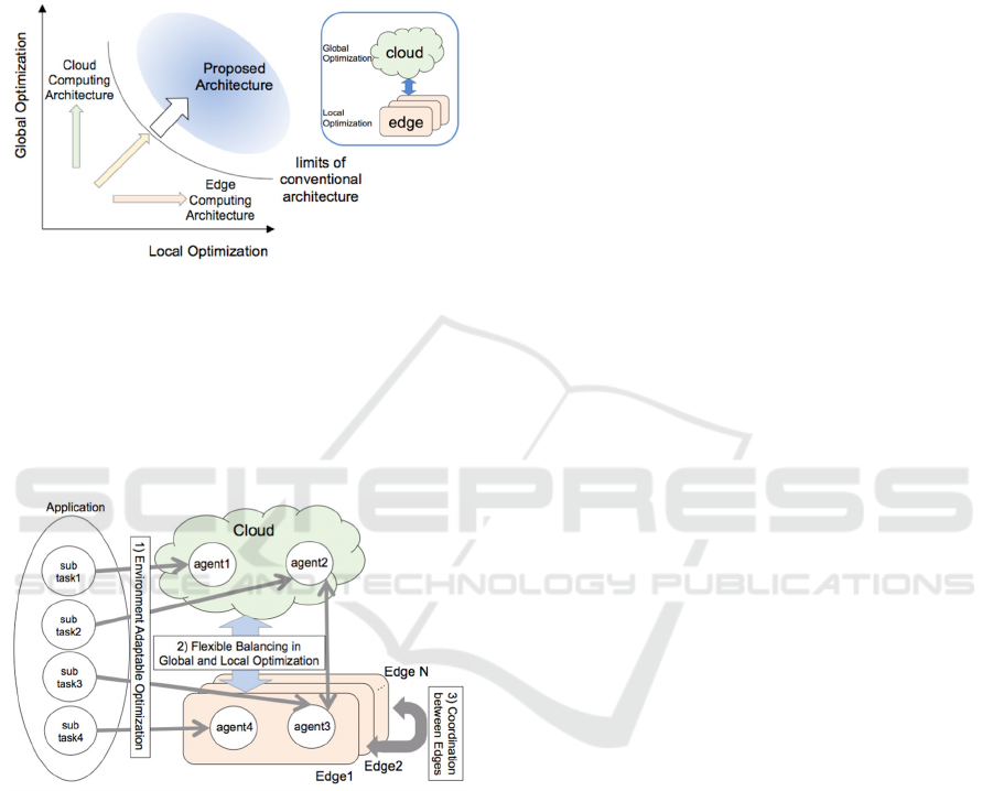
In our architecture, we propose a balancing
optimization mechanism with the collaboration of
both the global and the local subtasks. The goal of
this mechanism is to achieve total optimization of
the system, as shown in Figure 3.
Figure 3: Balancing Cloud and Edge Performances.
3.2 Architecture
Figure 4 shows the proposed architecture. An
application is divided into multiple subtasks that are
assigned as agents to the cloud or edges according to
their characteristics.
Figure 4: Multi-agent based Architecture of Flexible IoT-
EC.
Subtasks typically use autonomous distributed
multi-agency technology. When necessary, agents
can move from the cloud to the edges, from one
edge to another, etc.
When an application is divided into subtasks and
distributed to the cloud and the edges, it is necessary
to have a mechanism that allows the entire system to
work properly. If all information that determines the
behavior of the entire system is gathered in the cloud,
then, the optimization and control functions can only
be executed in the cloud. In many cases, such
information is dispersed throughout the system and
it is difficult for a single agent in the cloud to control
the entire system. When such agents exist both in the
cloud and on the edges, then, the agents need to
collaborate so that the system can balance properly
both in the cloud and at the edges. With the
mechanisms described above, our proposed system
can overcome the challenges encountered when
implementing IoT-EC.
3.3 Formulation
To balance the optimization of the total application,
the cloud and edge subtasks need to communicate
and agree on the details of the optimization process.
We will explain this situation with formalization.
Variables:
All the parameters that affect the system behavior
are described as variables
1
.
The variables
are classified according to the
accessible nodes: from the cloud, from the edges,
and from both.
is a variable used to alter cloud
behavior only.
is a variable used to alter the edge
behavior only.
is a shared variable that is used to
alter both the cloud and the edge systems.
=
,
,⋯
; from cloud
=
,
,⋯
; from edges
=
,
,⋯
; from both (1)
Cost Function:
We merge various indicators that are used to
evaluate the system behavior into one evaluation
function. We call this evaluation function a cost
function.
,
; for cloud
,
; for edge
,
,
=
,
+
∗
,
; for both cloud and edge (2)
Strictly speaking,
,
are different for
each edge, but we use the same designation
,
to make the expression easier to read.
,
and
,
are calculated
only in the cloud or the edges, respectively.
Consequently, the total optimization cannot be
calculated in one place. Thus, we need a mechanism
to obtain the optimal values step by step through
communicating between the cloud and the edges.
,
,
is the total cost function and the
total optimization is defined to minimize this cost
function under all the constraints. k is a parameter
Flexible IoT Edge Computing System to Solve the Tradeoff of Optimal Route Search
217

for ensuring proper balancing of the processing done
in the cloud and at the edge. Although, here the total
cost is assumed to be a linear equation of
,
and
,
, it may be a higher
order equation depending on the system.
Optimization:
Though not all variables can be freely changed, there
are some constraints (ex. 0<
<
+
).
Therefore, the system optimization is paraphrased as
a problem of minimizing the cost function under
certain constraints described below.
Global Optimization (Cloud):
,
,
,
Local Optimization (Edge):
,
,
,
Total Optimization:
,
,
,
,
,
,
4 SIMULATION IN THE ROUTE
SELECTION SYSTEM
This section discusses an evaluation of “Flexible IoT
edge system” through simulation in the route
selection system under intelligent transport systems
(ITS). This simulation confirms whether
optimization of cloud and edge optimization can be
improved by the proposed optimization method and
does not consider communication delay and other
influences accompanying the IoT system.
4.1 ITS and Route Selection System
ITS is a system that receives and transmits
information between people, roads, and cars. This is
a large-scale IoT system with clouds that aggregate
and process information from these edges (Usha and
Rukmini, 2016;
Peraković, Husnjak and Cvitić, 2014).
In this research, the evaluation was done by applying
the proposed architecture to a relatively simple route
selection system.
The route selection system selects the best route
from multiple routes. In our simulation, there were
two routes only. The edge optimization was to
minimize the travel time to the destination. The
purpose of cloud optimization is to minimize traffic
jam and the travel time of individual cars was not
considered.
4.2 Traffic Simulation
4.2.1 Optimal Velocity Model
In this simulation, car movements were simulated
using Optimal Velocity (OV) model (Bando et al.,
1995). The idea of OV model is as follows.
• A car will keep the maximum speed with enough
distance to the next car.
• A car tries to run with an OV determined by a
distance to the next car.
The basic equation is as follows,
=
=
−
−
(3)
where
represents the position and
the velocities
for each
.
The parameter 'a' is a sensitivity denoting the
speed of the response. In this simulation, 'a' is a
random number between 0.5 and 2.0. Each car has
its own fixed parameter 'a
j
'.
The function V(x) denotes the OV determined by
inter-vehicle distance. Here we take the following
tanh() type function as V(x).
=
×
ℎ
2.0
+ℎ4.0×
−
+2.0
ℎ
2.0
(4)
where maxspeed is the maximum speed of each path.
distMax is enough distance with which a car can
drive at the maxspeed. In the simulation, we set the
distMax as 100 m.
4.2.2 Fluctuation
The main cause of traffic congestion is caused by an
unintended deceleration at the sag curve (Nishinari,
2006). So a fluctuation was introduced to make the
simulation to appear like a real-life situation. In this
simulation, the speed of the car decreased randomly
by 20% with 25% probability.
4.2.3 Inter-vehicular Time
A car started at an appropriate inter-vehicular time
from the start point, reached the goal point and
stopped. We used this inter-vehicular time as a
parameter to change the density of the cars. When
distMax was 100 m and maxspeed was 40km/h, i.e.,.,
11.1 m/s, the car can run at maxspeed if the time
IoTBDS 2019 - 4th International Conference on Internet of Things, Big Data and Security
218
interval is more than about 9 seconds ( 100
11.1
⁄
9).
When the inter-vehicular time was smaller than 9
s, the speed of the car decreased and traffic jam
might happen just after a while from the start point.
In this situation, keeping the same inter-vehicular
time and continuing to put in more cars will result in
a situation whereby the distance between vehicles
becomes too short. Because this is not realistic, in
the simulation we conducted, the start of the next car
was suspended if the inter-vehicle distance was less
than 2 m. The start of the next car was resumed
when the distance exceeded 2 m. Therefore, the
actual inter-vehicle time was not necessarily the
same as the pre-defined value, but it may be larger
than that.
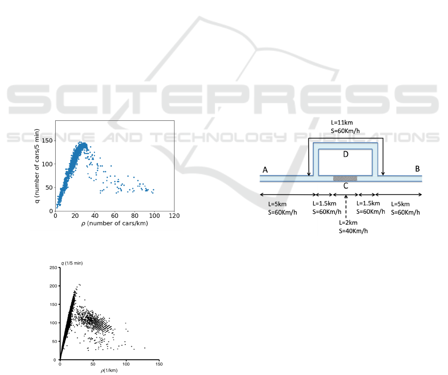
4.2.4 Confirmation of Validity of the
Simulation
With the above method, we check to what extent the
actual traffic jam can be reproduced through this
simulation. As shown in Figure 5, we draw a graph
of density and flow rate with random inter-vehicular
time. This graph is a fundamental diagram for
examining the state of traffic (Greenshields et al.,
1935), with the x-axis showing the car's density and
the y-axis showing the car's flow rate.
Figure 5: Traffic Simulation.
Figure 6: Typical fundamental diagram of the relation
between vehicle density and flow rate for one-month data
measured at a point on a freeway.
Figure 6 is an actual one-month data measured
by the Japan Highway Public Corporation
(Sugiyama, 2008).
In a density and flow rate graph, a concentrated
linear part on the left side shows a state in which
cars are flowing without congestion. A spread part
on the right side shows a congestion state. Our
simulation graph shows both states. Although the
graph is not exactly the same as the actual graph, we
evaluate it to be sufficient for our purpose.
4.3 Traffic Simulation to Confirm the
Effectiveness of the Proposed
Method
With our proposed architecture, the total system
optimization is integrated into the edge and cloud
optimizations. In the subsection, we would confirm
the feasibility of the proposed method.
4.3.1 Route Selection Simulation
The map shown in Figure 7 was used to conduct the
simulation. In this simulation, cars moved from
point A to point B. There were 2 routes, one is A to
C to B (route0), the other is A to D to C (route1).
When a car ran with maximum speed, the travel time
of route0 was shorter than that of route1.
Figure 7: The Simulation Map.
Traffic Jam Rate:
In this simulation, when the speed of one car was
less than half the maximum speed of the path, we
labeled the car to be in a traffic jam state. The traffic
jam rate is defined as a ratio of cars in a traffic jam
state to all the moving cars.
Edge Optimization:
With edge optimization, each car estimated the
travel time of every route and selects a minimum
travel time route. Each car could get the average
speed of each path in the designated route at that
time and calculated the estimated time when the car
Flexible IoT Edge Computing System to Solve the Tradeoff of Optimal Route Search
219
arrived the intersection. They could not predict
future changes.
Cloud Optimization:
With cloud optimization, we tried to reduce the
overall traffic jam rate. We did not consider the
travel time of individual cars.
If every path was not
going to get congested, we selected the shorter
arrival time.
No Optimization:
For the purpose of comparison, we also simulated
the results without rerouting, i.e., every car ran
through route0.
Parameters:
The simulation was conducted by changing the start
inter-vehicular time from 6.0s to 12.0s.
Because the maximum speed of the path was
60km/h (16.7 m/s) and 40km/h (11.1 m/s) and
distMax was 100 m, when all the cars ran at the
same speed with distMax distance, the inter-vehicle
time at each speed was 6.0s and 9.0s, respectively.
When the influence of the fluctuation of the vehicle
speed was considered, it became 6.3s and 9.5s
respectively.
The simulation started with no car in the system.
The calculation was done after the first car arrived
the goal point. The simulation continued until 2000
cars started from the start point.
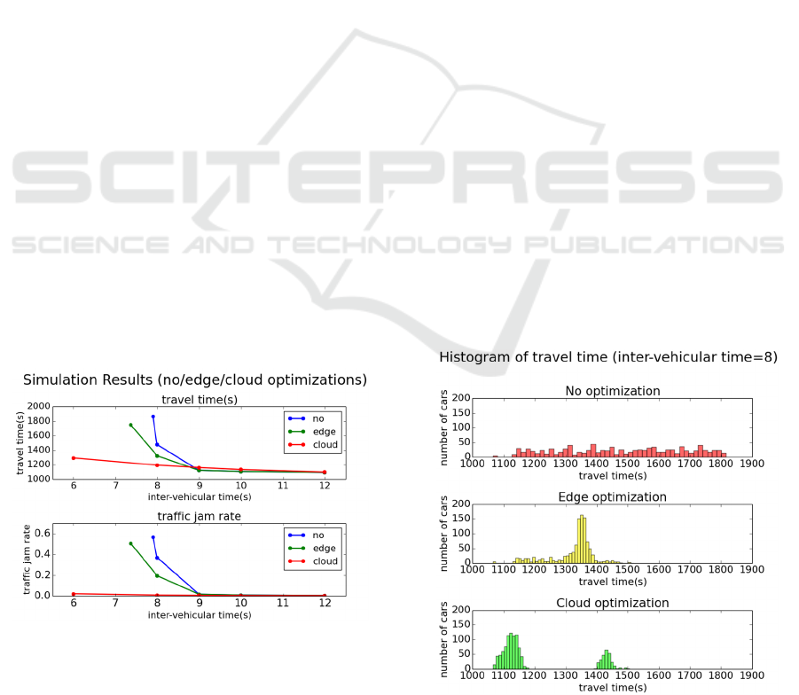
4.3.2 Simulation Results
All the results were shown in Figure 8. The average
travel time and the average traffic jam rate for each
cases. Each optimization results are explained
below.
Figure 8: Simulation Results with 3 Optimizations.
When there was no optimization, all the cars ran
through route0. The travel time, in the case where
there was no traffic jam and the cars could run at the
maximum speed, was 1010 seconds by taking
fluctuation into consideration are as follows.
60km/h section: 13km / 60km/h / 0.95
= 821.1 seconds
40km/h section: 2km / 40km/h / 0.95
=189.5seconds
Total: 821.1 + 189.5 = 1010.6 seconds
When the inter-vehicular time was under 9
seconds, the traffic jam states began and the travel
time increased. This happened in the edge
optimization case but the traffic jam rate was smaller
and the travel time was smaller than no optimization
case.
In the cloud optimization, the goal of lowering
the traffic jam rate was realized and as a result, the
average travel time was kept low.
Regarding the average travel time, edge
optimization was better than the no optimization
case in almost all the cases. Cloud optimization had
the worst performance when the inter-vehicular time
was more than 9 s. But when the inter-vehicular time
was less than 8, it had better numbers than the edge
optimization and no optimization.
To investigate this state in more detail, a
histogram of travel times when the inter-vehicular
time was 8 s is shown in Figure 9.
Looking at the histogram of the travel time of
cars, we can see that the patterns are distinctly
different in the three results especially in the case of
cloud optimization where there are 2 peaks in the
histogram which means that the improved average
travel time was realized under the sacrifice of some
cars with long travel time.
Figure 9: Histogram of Travel Time.
IoTBDS 2019 - 4th International Conference on Internet of Things, Big Data and Security
220
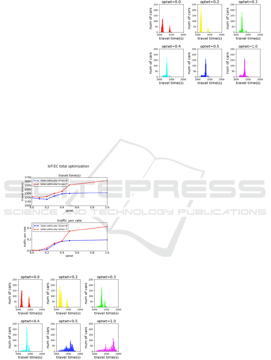
4.3.3 Simulation Results with Proposed
IoT-EC Optimization
Next, we simulate the proposed IoT-EC total
optimization. As explained in subsection 3.3, with
the proposed total optimization, we added edge and
cloud optimizations with appropriate weight. Since
we do not know the appropriate weight yet, we will
change the weights and check the change in the
travel time and the traffic jam rate.
In this simulation, the total cost is calculated
using the following equation.
=
1−
∙
+∙
0.0 1.0
(5)
optwt means the optimization weight. When
optwt is 0.0, this cost
t
(v) becomes the same as the
cloud cost function cost
c
(v). When optwt is 1.0, this
cost
t
(v) becomes the edge cost function cost
e
(v). The
simulation was conducted with inter-vehicle time set
at 7.0s and 8.0s. Figure 10 shows the results.
Figure 10: Simulation of IoT Edge optimization.
Figure 11: Histogram of drive time with total IoT-EC
optimization (inter-vehicular time = 7).
Figure 12: Histogram of travel time with total IoT-EC
optimization (inter-vehicular time = 8).
Traffic jam rate is the minimum value obtained
using the cloud optimization (optwt = 0.0). The
travel time is the minimum value at an optwt value
ranging from 0.1 to 0.2.
Figure 11 and Figure 12 show the histogram of
the travel time. As the optwt increases, we can see
that the two peaks obtained using the cloud
optimization shifts to one peak with the edge
optimization.
5 DISCUSSIONS
The purpose of this simulation is to confirm if the
best system optimization is fulfilled with a
combination of edge and cloud optimizations. The
purpose of edge optimization is to reduce travel time
while the purpose of cloud optimization is to
decrease the traffic jam rate. Concerning the average
travel time, a combination of edge and cloud
optimizations produces the best average travel time
with a suitable weight value. For the traffic jam rate,
the best rate was produced using the cloud and the
combinational optimizations with appropriate weight
value.
The edge optimization produced a better
performance compared to the case where there was
no optimization. However, with short inter-vehicular
time, cloud optimization produced a better average
travel time performance. This suggests that there
could be a better calculation method for optimizing
arrival time.
Cloud optimization produced a better traffic jam
rate. At the same time, it also produced a better
travel time with low inter-vehicular time. Looking at
the details of the cloud optimization, we can observe
two peaks in the histogram of the travel time. This
means that the improved average travel time was
Flexible IoT Edge Computing System to Solve the Tradeoff of Optimal Route Search
221

realized at the expense of some of the cars with long
travel time. It would be necessary to incorporate the
measure of fairness into the cost function.
Alternatively, a method of changing the parameter
of selection according to the degree of urgency of
the car is needed.
In the simulation conducted, we found that by
choosing appropriate weights, it is possible to find
optimal values that could not be obtained
independently by combining edge and cloud
optimizations. However, the appropriate weights are
merely a result of the range considered in this
simulation and, thus, the application range of the
proposed method needs to be confirmed using a
wider range of simulations.
6 SUMMARY
In this paper, the effectiveness of the IoT edge
system, which aims to optimize the whole system,
was examined using a simple route selection system
by appropriately combining edge and cloud
optimizations. In the case of a simple route selection
algorithm, the optimal travel time was realized based
on the cost function of the proposed optimization
method.
Our future work would focus on confirmation of
the effects of the proposed system in an optimal
route searching system that is closer to the real
system. We also plan to extend our research to other
IoT application domains.
REFERENCES
Abdelshkour, M., 2015. IoT, from Cloud to Fog
Computing. [Online] Available from:
http://blogs.cisco.com/perspectives/iot-from-cloud-to-
fog-computing [Accessed 9
th
Feb. 2019].
Al-Fuqaha, A., Guizani, M., Mohammadi, M., Aledhari M.
and Ayyash, M., 2015. Internet of Things: A Survey on
Enabling Technologies, Protocols, and Applications. In
IEEE Communications Surveys & Tutorials, vol. 17, no.
4, pp. 2347-2376, Fourthquarter 2015.
Bando, M., Hasebe, K., Nakayama, A. and Shibata, A.,
1995. Dynamical model of traffic congestion and
numerical simulation. In Physical Review E, vol. 51,
no. 2, pp. 1035-1042, Feb. 1995.
Greenshields, B., Channing, W., Miller, H., 1935. A study
of traffic capacity. In Highway research board
proceedings, no. 14, pp.448-477.
Kitagami, S., Yamamoto, M., Imamura, M., Kambe, H.,
Koizumi, H., Suganuma, T., 2013. An M2M Data
Analysis Service System based on Open Source
Software Environment. In The transactions of IEEJ.
C, vol. 133, no. 8, pp. 1521-1528, Aug. 2013, (in
Japanese).
Kitagami, S., Thanh, V. T., Bac, D. H., Urano, Y.,
Miyanishi, Y., Shiratori, N., 2016. Proposal of a
Distributed Cooperative IoT System for Flood
Disaster Prevention and its Field Trial Evaluation. In
International Journal of Internet of Things, vol. 5, no.
1, pp. 9-16, Apr. 2016.
Lopez, P. G., Montresor, A., Epema, D., Datta, A.,
Higashino, T., Iamnitchi, A., Barcellos, M., Felber, P.
Riviere, E., 2015. Edge-centric Comuting: Vision and
Challenges. In ACM SIGCOMM Computer Communi-
cation Review, vol. 45, no. 5, pp. 37-42, Oct. 2015.
Nishinari, K., 2006. Study on Congestion. Shincho
Sensho, Tokyo, (in Japanese).
Ogino, T., Kitagami, S., Suganuma, T., Shiratori, N.,
2018. A Multi-agent Based Flexible IoT Edge
Computing Architecture Harmonizing Its Control with
Cloud Computing. In International Journal of
Networking and Computing, vol. 8, no. 2, pp. 218-239.
Peraković, D., Husnjak, S. and Cvitić, I., 2014. IoT
Infrastructure as a Basis for New Information Services
in the its Environment. In Proc. 2014 22nd
Telecommunications Forum Telfor (TELFOR), Nov.
2014.
Ren, J., Guo, H., Xu and C., Zhang, Y., 2017. Serving at
the Edge: A Scalable IoT Architecture Based on
Transparent Computing. In IEEE Network, vol. 31, no.
5, pp. 96-105.
Shi, W., Cao, J., Zhang, Q., Li, Y. and Xu, L., 2016. Edge
Computing: Vision and Challenges. In IEEE Internet
of Things Journal, vol. 3, no. 5, pp. 637-646.
Shiratori, N., Kitagami, S., Suganuma, T., Sugawara, K.
and Shimamoto, K., 2017. Latest Development of IoT
Architecture. In The Journal of the Institute of
Electronics, Information and Communication
Engineers, vol. 100, no. 3, pp. 214-221, Mar. 2017 (in
Japanese).
Suganuma, T., Uchibayashi, T., Kitagami, S., Sugahara
K., Shiratori, N., 2016. Proposal of An Environment
Adaptive Architecture for Flexible IoT. In IEICE
technical report, vol.116, no.231, pp.13-18, Sep. 2016
(in Japanese).
Sugiyama, Y., Fukui, M., Kikuchi, M., Hasebe, K.,
Nakayama, A., Nishinari, K., Tadaki, S. and Yukawa
S., 2008. Traffic Jams Without Bottlenecks -
Experimental Evidence for the Physical Mechanism of
the Formation of a Jam. In New Journal of Physics,
vol. 10, no. 3, pp. 033001.
Usha Devi, Y. and Rukmini, M.S.S., 2016. IoT in
connected vehicles: Challenges and issues—A review.
In Proc. 2016 International Conference on Signal
Processing, Communication, Power and Embedded
System (SCOPES), Oct. 2016.
Yang, Z., Yue, Y., Yang, Y., Peng, Y., Wang, X. and Liu,
W., 2011. Study and application on the architecture
and key technologies for IOT. In 2011 International
Conference on Multimedia Technology, Hangzhou,
2011, pp. 747-751.
IoTBDS 2019 - 4th International Conference on Internet of Things, Big Data and Security
222
