A Study of Joint Policies Considering Bottlenecks and Fairness
Toshihiro Matsui
Nagoya Institute of Technology, Gokiso-cho Showa-ku Nagoya 466-8555, Japan
Keywords:
Multiagent System, Multi-objective, Reinforcement Learning, Bottleneck, Fairness.
Abstract:
Multi-objective reinforcement learning has been studied as an extension of conventional reinforcement learn-
ing approaches. In the primary problem settings of multi-objective reinforcement learning, the objectives
represent a trade-off between different types of utilities and costs for a single agent. Here we address a case of
multiagent settings where each objective corresponds to an agent to improve bottlenecks and fairness among
agents. Our major interest is how learning captures the information about the fairness with a criterion. We
employ leximin-based social welfare in a single-policy, multi-objective reinforcement learning method for
the joint policy of multiple agents and experimentally evaluate the proposed approach with a pursuit-problem
domain.
1 INTRODUCTION
Reinforcement learning (Sutton and Barto, 1998)
has been studied for optimization methods of single
and multiple agent systems. While conventional re-
inforcement learning methods address optimization
problems with single objectives, multi-objective re-
inforcement learning (Liu et al., 2015) solves an ex-
tended class of problems for optimal policies to si-
multaneously improve multiple objectives.
In the primary problem settings of multi-objective
reinforcement learning, the objectives represent a
trade-off between different types of utilities and costs
for a single agent. For example, in a setting where a
robot collects items from its environment, the objec-
tive is the number of collected items, and other ob-
jectives are energy consumption and risk avoidance.
Those objectives are represented as a multi-objective
maximization/minimization problem.
Similar to the solution methods for conventional
multi-objective optimization problems, several scalar-
ization functions and social welfare criteria are ap-
plied to select one of optimal solutions, since many
Pareto optimal (or quasi-optimal) policies exist in
general cases. A fundamental scalarization function
is the weighted summation for objectives. Other
non-linear functions are also applied, including the
weighted Tchebycheff function and its variants (Mof-
faert et al., 2013). While applying scalarization func-
tions in learning processes optimizes a single policy,
different approaches apply other minimization filters
so that multiple policies are simultaneously optimized
with a memory consumption.
Even though most studies of multi-objective re-
inforcement learning address a single agent domain,
the objectives can also be related to multiple agents.
A simple representation of such problems is the op-
timization of the joint policies of multiple agents.
In this case, opportunities can be found for employ-
ing different scalarization functions and social wel-
fare criteria to improve fairness among the agents. If
the learning captures the information of the fairness,
there might be additional opportunities for multiagent
reinforcement learning with approximate decomposi-
tions of state-action space, while different approaches
also exist, such as the methods to converge equilib-
ria (Hu and Wellman, 2003; Hu et al., 2015; Awheda
and Schwartz, 2016).
Several criteria represent fairness or inequal-
ity. The maximization of leximin (Bouveret and
Lemaˆıtre, 2009; Greco and Scarcello, 2013; Matsui
et al., 2018a; Matsui et al., 2018c; Matsui et al.,
2018b) is an extension of maximin that improves
the worst case utility and fairness. It also slightly
improves the total utility. Leximin is based on the
lexicographic order on the vectors whose values are
sorted in ascending order. Several studies of combi-
national optimization problems show that the conven-
tional optimization criterion is successfully replaced
by the leximin criterion. Other inequality measure-
ments could also be applied to this class of problems,
while several modifications to improvethe total utility
80
Matsui, T.
A Study of Joint Policies Considering Bottlenecks and Fairness.
DOI: 10.5220/0007577800800090
In Proceedings of the 11th International Conference on Agents and Artificial Intelligence (ICAART 2019), pages 80-90
ISBN: 978-989-758-350-6
Copyright
c
 2019 by SCITEPRESS – Science and Technology Publications, Lda. All rights reserved

or cost with trade-offs are necessary for pure unfair-
ness criteria.
In this work, we focus on single-policy, multi-
objective reinforcement learning with leximax, which
is a variant of leximin for minimization problems.
Our primary interest is how different types of social
welfare can be applied to a multi-objective reinforce-
ment learning method. For the first study, we em-
ploy a simple class of pursuit problems with multiple
hunters and a single target. We first consider a de-
terministic setting and apply a dynamic programming
method. Next we investigate how the approach is af-
fected by a non-deterministic setting and experimen-
tally evaluate the effects and influences of the leximax
criterion.
The rest of our paper is organized as follows. In
the next section, we describe several backgrounds
to our study. We address an approach that applies
the leximax criterion to multi-objective Q-learning
scheme for joint actions among agents in Section 3.
Our proposed approach is experimentally evaluated
in Section 4 and several discussions are described in
Section 5. We conclude in Section 6.
2 PREPARATION
2.1 Reinforcement Learning and
Multiple Objectives
Reinforcement learning is a unsupervised learning
method that finds the optimal policy, which is a se-
quence of actions in a state transition model. In
this work, we focus on Q-learning based methods
as fundamental reinforcement learning methods. Q-
learning consists of set of states S, set of actions A,
observed reward/cost values for actions, evaluation
values Q(s, a) for each pair of state s ∈ S and action
a ∈ A, and parameters for learning. When action a is
performed in state s, a state transition is caused with
a corresponding reward/cost value based on an envi-
ronment whose optimal policy should be mapped to
Q-values.
For the minimization problem, a standard Q-
learning is represented as follows
Q(s, a) ← (1− α)Q(s, a) + α(c+ γ min
a
′
Q(s
′
, a
′
)) ,
(1)
where s and a are the current state and action, s
′
and
a
′
are the next state and action, and c is a cost value
for action a in state s. α and γ are the parameters of
the learning and discount rates.
In basic problems, complete observation of all of
the states without confusion is assumed so that the
learning process correctly aggregates the Q-values.
The Q-values are iteratively updated with action se-
lections based on an exploration strategy, and the val-
ues can be sequentially or randomly updated to prop-
agate them by dynamic programming.
Reinforcement learning is extended to find a pol-
icy that simultaneously optimizes multiple objectives.
For multiple objective problems, cost values and Q-
values are defined as the vectors of the objectives.
Learning rules are categorized into single and mul-
tiple policy learning. In single policy learning, each
Q-vector is updated for one optimal policy with a fil-
ter that selects a single objective vector. On the other
hand, multiple policy learning handles multiple non-
dominated objective vectors for each state-action pair
and selects a Pareto optimal (or quasi-optimal) pol-
icy after the learning, while it generally requires more
memory. We focus on single policy learning.
For a single policy with the social welfare of
weighted summation, multi-objective Q-learning is
represented as follows
Q(s, a) ← (1− α)Q(s, a)+α(c+γ minws(v, Q(s
′
, a
′
)))
(2)
’minws’ is a minimization operator based on a
weighted summation with vector v
argmin
Q(s
′
,a
′
) for a
′
v · Q(s
′
, a
′
) (3)
In general settings, multiple objectives represent
several trade-offs, such as the number of collected
items and the energy consumption of a robot. Their
main issue is how to obtain the Pareto optimal poli-
cies. On the other hand, we address a class of multi-
objective problems where each objective corresponds
to the cost of an agent.
2.2 Criteria of Bottlenecks and Fairness
There are several scalarization functions and social
welfare criteria that select an optimal objective vec-
tor (Sen, 1997; Marler and Arora, 2004).
Summation
∑
K
i=1
v
i
for objective vector v =
[v
1
, · · · , v
K
] is a fundamental scalarization function
that considers the efficiency of the objectives. The
minimization of the (weighted) summation is Pareto
optimal. However, it does not capture the fairness
among the objectives.
The minimization of maximum objective value
max
K
i=1
v
i
, called minimax, improves the worst case
cost value. However, the minimization of the
(weighted) maximum value is not Pareto optimal. A
variant with the tie-breaking of the weighted maxi-
mum value with the weighted summation is called the
augmented weighted Tchebycheff function. The min-
imization with this scalarization is Pareto optimal.
A Study of Joint Policies Considering Bottlenecks and Fairness
81

We focus on a criterion called leximax that resem-
bles leximin for maximization problems. Leximin is
defined as the dictionary order on objective vectors
whose values are sorted in ascending order (Bouveret
and Lemaˆıtre, 2009; Greco and Scarcello, 2013; Mat-
sui et al., 2018a; Matsui et al., 2018c). The leximax
relation is defined as follows with sorted objective
vectors v and v
′
where the values in their original ob-
jective vectors are sorted in descending order.
Definition 1 (leximax). Let v = [v
1
, · · · , v
K
] and v
′
=
[v
′
1
, · · · , v
′
K
] denote sorted objective vectors whose
length is K. The order relation, denoted with ≻
leximax
,
is defined as follows. v ≻
leximax
v
′
if and only if
∃t, ∀t
′
< t, v
t
′
= v
′
t
′
∧ v
t
> v
′
t
.
The minimization on leximax improves the worst
case cost value (bottleneck value) and the fairness
among the cost values.
We employ the Theil index, which is a well-
known measurement of inequality. Although this
measurement was originally defined to compare in-
comes, we use it for cost vectors.
Definition 2 (Theil Index). For n objectives, Theil in-
dex T is defined as
T =
1
n
∑
i
v
i
¯v
log
v
i
¯v
, (4)
where v
i
is the utility or the cost value of an objective
and ¯v is the mean utility value for all the objectives.
The Theil index takes a value in [0, logn], since it
is an inverted entropy. When all the utilities or cost
values are identical, the Theil index value is zero.
3 JOINT POLICIES
CONSIDERING BOTTLENECKS
AND EQUALITY
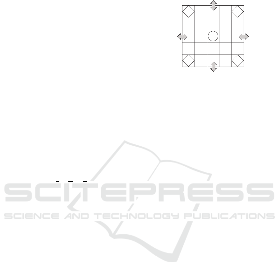
3.1 Example Domain
We employ a simplified pursuit game with four
hunters and one target in a torus grid world (Figure 1).
The hunters should cooperatively capture the target
reducing the number of moves, while their individual
move cost values are defined as multiple objectives.
To handle joint states and joint actions with a sin-
gle table and sufficiently scan the state-action space,
hunters take only one of two actions: stop or move.
When a hunter selects a move, it advances to a neigh-
boring cell in four directions to decrease its distance
to the target. If all the hunters move, the target will
be captured in relatively few steps. However, the
moves of hunters cause costs. The target escapes from
t
h
0
h
1
h
2
h
3
Figure 1: Pursuit game with four hunters h
i
and one target
t.
hunters. It moves to a neighboring cell to maximize
its distance to the nearest hunter.
To eliminate noise from the stochastic process and
the limited sensing, we first choose a deterministic
process with a complete observation. The hunters and
the target deterministically act with deterministic tie-
breaking. The hunters know the location of the tar-
get. We address the problem of joint states and joint
actions as the first study. The deterministic process is
replaced by a non-deterministicprocess with random-
ness in the tie-breaking of target actions later.
Targets and hunters stay in the current cell or move
to adjoining cells in either vertical or horizontal direc-
tions. The goal states are cases where one of hunters
and the target are in the same cell. A joint policy is
a sequence of joint actions of hunters from an initial
state to a goal state.
The target moves to cells to maximize its min-
imum distance to the hunters. In the deterministic
case, the directions are prioritized in the following or-
der: upward, downward, left and right. If there are no
improvements, the target stays in the current cell. In
the non-deterministic case, ties are randomly broken
with uniform distribution.
A hunter moves to cells to minimize its distance
to the target. Here vertical directions are priori-
tized over horizontal directions. The hunters employ
this tie-break rule in both the deterministic and non-
deterministic cases. A move of a hunter causes a cost
value of one, while the hunter can remain in the cur-
rent cell at a cost value of zero. To avoid cases where
no hunter moves, infinity cost values are set to all
hunters for such a joint action.
We encoded the joint states and actions as follows.
For each hunter, a pair of vertical and horizontal dif-
ferences between the coordinates of the hunter and the
target represent their relative locations. The differ-
ence of the minimum distance in the torus grid world
is employed. The relative locations are combined for
all hunters. Therefore, for grid size g, two types of
actions, and four hunters, the number of joint state-
ICAART 2019 - 11th International Conference on Agents and Artificial Intelligence
82

actions is (g× g× 2)
4
.
The goal of the reinforcement learning is to find
the optimal (or quasi-optimal) policy that reduces the
total cost values with an appropriate criterion. In a
common problem setting, the optimal joint policy can
be defined as the joint policy which minimizes the to-
tal number of moves for all hunters. Namely, the sum-
mation is employed as the criterion to aggregate cost
values for all hunters. As the first study, we focus
on centralized reinforcement learning methods, while
there might be opportunities to decompose the prob-
lem into multiple approximated ones for agents.
We address the joint policies that improve the fair-
ness among the total cost values of individual hunters
with the leximax criterion, while a common policy
improves the total cost values for all of them. In the
case of the minimization of leximax, the bottleneck
is the maximum number of moves among individual
hunters, and unfairness can also be defined for the
number of moves among the hunters. Both should
be reduced with the optimal (or quasi-optimal) policy.
Our major interest is how such information is mapped
in a Q-table of a reinforcement learning method.
3.2 Multi-objective Deterministic
Decision Process
We start from a deterministic domain to consider
the fundamental operations of the learning, which
is identical as the dynamic programming for path-
finding problems. Next we turn to the case of a non-
deterministic domain.
3.2.1 Basic Scheme
We focus on the opportunities of the optimal Q-table
for the leximax criterion. Therefore, we assume an
appropriate exploration strategy and simply employ a
propagation method that resembles the Bellman-Ford
algorithm as an offline learning method. The update
of the Q-table will eventually converge after a suffi-
cient number of propagation operations. We eliminate
statistic elements (i.e. the learning and discount rates)
for the deterministic process.
A common deterministic update rule for single ob-
jective problems is represented as follows
Q(s, a) ← c+ min
a
Q(s
′
, a
′
) . (5)
A deterministic update rule for multi-objective
problems with summation scalarization is similarly
represented
Q(s, a) ← sum(c) + min
a
Q(s
′
, a
′
) , (6)
s
g
s
1
s
0
0
1
1
0
0
1
0
2
1
1
max(0,1)=1
max(1,0)=1
cost
cost
Q(s
0
,a
0
)
max(0,2)=2
max(1,1)=1
a
0
a
1
'
a
1
(for a
1
)
(for a
1
' )
Figure 2: Incorrect minimax aggregation.
where sum(c) is a summation scalarization func-
tion that returns the summation of the values in cost
vector c. We do not use any weighted scalarization
functions, because we assume that the hunters have
the same priority. This rule is equivalent to Equa-
tion (2) with α = 1, γ = 1, and all-one vector v, al-
though the Q-values in Equation (6) are scalar. We
refer to this rule as single objective learning for multi-
objective problems with summation scalarization in
experimental evaluations.
On the other hand, Equation (2) with α = 1, γ = 1,
and all-one vector v,
Q(s, a) ← c + argmin
Q(s
′
,a
′
) for a
′
v · Q(s
′
, a
′
) , (7)
is a basic scheme of multi-objective learning for a
deterministic process, where the Q-vectors aggregate
the cost vectors of the optimal policy. For different
criteria, the minimization and the aggregation must
be modified.
3.2.2 Applying Scalarization based on leximax
Although one can think that the minimization opera-
tor is simply replaced with other scalarization criteria,
such an assumption is incorrect in general cases. The
summation case is correct. Figure 2 shows an aggre-
gation of two objectives with an incorrect minimax
operation. In this example, actions a
1
and a
′
1
cause
transitions from state s
1
to goal state s
g
with cost vec-
tors [0, 1] and [1, 0], respectively. Since the maximum
value in these two cost vectors is one, they cannot be
distinguished by the minimax. On the other hand, pre-
vious action a
0
causes a transition from state s
0
to s
1
with cost vector [0, 1]. Therefore, Q(s
0
, a
0
) takes [0, 2]
for action a
1
, while it takes [1, 1] for a
′
1
.
The minimum cost value for Q(s
0
, a
0
) is different
for subsequent actions even though the decision pro-
cess is deterministic. This also means that there is
no information to select the optimal policy. This is
a problematic situation, while it might be mitigated
in non-deterministic cases. Since leximax is an ex-
A Study of Joint Policies Considering Bottlenecks and Fairness
83

tension of maximum scalarization, the same problem
exists.
To avoid that problem, we apply a minimization
operation to the aggregated cost vectors. For the min-
imization of leximax, the update rule is represented as
follows
Q(s, a) ← min
leximax
a
′
(c + Q(s
′
, a
′
)) , (8)
where c is a cost vector for current action a. The vec-
tors are compared in the manner of leximax.
We must also modify the action selection after the
learning process. In the original action selection, the
action of the minimum Q-value is simply selected.
However, for the modified case, such an action might
be incompatible with the previous action, since it is
selected without considering the aggregation process.
To ensure compatibility among actions, we introduce
the following condition
Q(s
−
, a
−
) = c
−
+ Q(s, a) , (9)
where Q(s
−
, a
−
) is the Q-vector for the previous state
and action and Q(s, a) is the Q-vector for the current
state and action. c
−
is the cost vector for previous ac-
tion a
−
. Namely, the actions in the current state are
filtered by this condition, and the optimal action is se-
lected from the filtered ones. In the initial state, the
action selection is unfiltered, since there is no previ-
ous action. The procedure of action selection is sum-
marized as follows.
1. For initial state s, select optimal action a =
argmin
leximax
a
′
Q(s, a
′
).
2. Perform action a and transit to the next state. Save
Q(s, a) and cost c for a as Q(s
−
, a
−
) and c
−
.
3. Terminate when the goal state is achieved.
4. For current state s, select optimal action
a = argmin
leximax
a
′
(c
−
+ Q(s, a
′
)) such that
Q(s
−
, a
−
) = c
−
+ Q(s, a
′
).
5. Return to 2.
With these modifications, the objectivesare aggre-
gated and compared without incorrect decomposition
of the summation of vectors, although we need addi-
tional computations to maintain compatibility among
actions.
3.3 Non-deterministic Domain
The update rules for the deterministic process are ex-
tended for the non-deterministic case. For the case
of summation, the update rule is the case of Equa-
tion (2) when weight vector v is an all-one vector.
The rule is equivalent to the following rule with sum-
mation scalarization
Q(s, a) ← (1− α)Q(s, a) + α(sum(c) + γmin
a
Q(s
′
, a
′
)))
(10)
The update rule in Equation (8) is modified for the
non-deterministic process.
Q(s, a) ← (1− α)Q(s, a) + α min
leximax
a
′
(c + γ Q(s
′
, a
′
))
(11)
Learning rate α is applied to a cost vector that
is minimized for aggregated vectors c + γ Q(s
′
, a
′
).
Discount rate γ can be identically generalized as the
original reinforcement learning process. Here we fix
the discount rate to one, since we focus on the fair-
ness among individual total cost values for hunters
and equally treat all action cost vectors.
We employ action selection similar to that for the
deterministic process. However, this is not straight-
forward, since the condition in Equation (9), which
maintains compatibility among actions, cannot be sat-
isfied due to statistic aggregation. Therefore, the con-
dition should be approximately evaluated consider-
ing the errors. Here we modify the condition us-
ing the leximax operator for the difference between
Q(s
−
, a
−
) and c
−
+ Q(s, a). Step 4 of the action se-
lection in Section 3.2.2 is replaced as follows.
• For current state s, select action a =
argmin
leximax
a
′
((c
−
+ Q(s, a
′
)) − Q(s
−
, a
−
)).
• Break ties with a = argmin
leximax
a
′
(c
−
+Q(s, a
′
)).
In general cases, the first rule will usually be
applied. The minimization of difference (c
−
+
Q(s, a
′
)) −Q(s
−
, a
−
) reduces the cost values that ex-
ceed the estimated values in the previous action se-
lection. Although such minimization might cause
over-estimations when several cost values are reduced
more than their necessary values, we prefer to take a
margin for the non-deterministic process. However,
such over-estimations might increase the total cost of
some hunters due to a mismatch.
3.4 Correctness and Complexity
In the case of a deterministic process with an appro-
priate minimization criterion and tie-breaking among
vectors, the learning process eventually converges to a
quasi-optimal vector. The minimum cost vector prop-
agates from the goal states to each state. We note that
a non-monotonicity might be found in an update se-
quence of Q-vector Q(s, a). However, it does not af-
fect the above learning process, since it always over-
writes the old Q-vectors. Therefore, each Q-vector
converges to the minimum vector in terms of the min-
imum leximax filtering.
On the other hand, no assurance exists that the ob-
tained policy is globally optimal in terms of the lex-
imax for the individual total cost values for hunters.
ICAART 2019 - 11th International Conference on Agents and Artificial Intelligence
84

Even though leximax aggregation is precisely decom-
posed with dynamic programming approaches in sev-
eral cases (Matsui et al., 2018a; Matsui et al., 2018c;
Matsui et al., 2018b), this is not the case. We assume
that fair policies are more easily improved than un-
fair policies when additional actions are aggregated.
This depends on the freeness of the problem that al-
lows such a greedy approach. Although this approach
is only a heuristic, it will reasonably work when there
are a number of opportunities to improve the partial
costs with previous actions in the manner of leximax.
For most non-deterministic cases, the learning
process will not converge. However, after a sufficient
number of updates with an appropriate learning rate,
the Q-vectors will have some statistic information of
the optimal policy similar to the case of a determinis-
tic process.
Since leximax employs operations with sorted
vectors, the computational overhead of the proposed
approach is significantly large. While our major inter-
est in this work is how the information of bottlenecks
and fairness is mapped to Q-values, the overhead
should be mitigated with several techniques, such as
the caching of sorted vectors in practical implementa-
tions.
4 EVALUATION
We experimentally evaluated our proposed approach
for deterministic and non-deterministic processes by
employing the example domain of the pursuit prob-
lem.
4.1 Settings
As shown in Section 3.1, we employ a pursuit prob-
lem with four hunters and one target. The grid size
of the torus world is 5× 5 or 7 × 7 grids for the de-
terministic domain, and the size is 5× 5 grids for the
non-deterministic domain due to the limitations of the
computation time of the learning process.
After the learning process, policy selection is per-
formed and the individual total cost values for the
hunters are evaluated. Here the total cost value cor-
responds to the total number of moves of each hunter.
In this experiment, the locations of the four hunters
are set to four corner cells (Figure 1). In the grid
world, it is identical to that the hunters are gathered
into an area. On the other hand, the initial locations
of the target are set to all the cells except the initial
locations of the hunters. We performed ten trials for
each setting and averaged their results.
We compared the following three methods.
• sum: a single objective reinforcement learning
method shown in Equation (6) and (10) that mini-
mizes the total cost for all the hunters.
• lxm: a multi-objective reinforcement learning
method that minimizes the individual total cost
values for all the hunters with the minimum lexi-
max filtering.
• sumlxm: a multi-objective reinforcement learning
method that minimizes the total cost for all the
hunters. However, the policy selection is the same
as ‘lxm’. Note that we employed update rules that
resemble Equations (8) and (11) by replacing the
filtering criterion to minimum summation, so that
the Q-vectors are compatible with ‘lxm’.
Here ‘sumlxm’ is employed to distinguish the ef-
fects of the Q-vectors for the minimum leximax ap-
proach from the action selection method.
4.2 Results
4.2.1 Deterministic Domain
We first evaluated the proposed approach for the de-
terministic decision process without any randomness
for the moves of the hunters and the target. The learn-
ing process repeatedly updated the Q-vectors for all
the joint state-action pairs, similar to the Bellman-
Ford algorithm. In the deterministic case, after a few
iterations of all the updates for all the Q-vectors, the
vectors converged. Due to the infinity cost vector for
the all-stop joint actions, there were no infinite cyclic
policies.
Table 1 shows the total cost values for different
methods in the 5× 5 world. The size of the joint state-
action space to be learned is (5× 5× 2)
4
= 6, 250, 000
for this problem. In a policy selection experiment,
there are 5 × 5 − 4 = 21 initial locations for the tar-
get and 210 instances for ten trials. The results show
that ‘sum’ minimizes the total cost for all the hunters
which is equivalent to the average cost. On the other
hand, ‘lxm’ minimizes the maximum total cost for the
individual hunters, and also reduces the values of the
Theil index, which is a criterion of unfairness. Since
there are trade-offs between efficiency and fairness,
the total (i.e. the average) cost for all hunters of ‘lxm’
is not less than that of ‘sum’.
The result of ‘sumlxm’, which is a combination
of the learning of ‘sum’ and the action selection of
‘lxm’, shows mismatches between the learning and
the action selection. It also reveals that both the learn-
ing and the action selection of ‘lxm’ havesome effects
in its improvements.
In addition, the policy length of ‘lxm’ is relatively
greater than that of ‘sum’. A possible reason is that
A Study of Joint Policies Considering Bottlenecks and Fairness
85

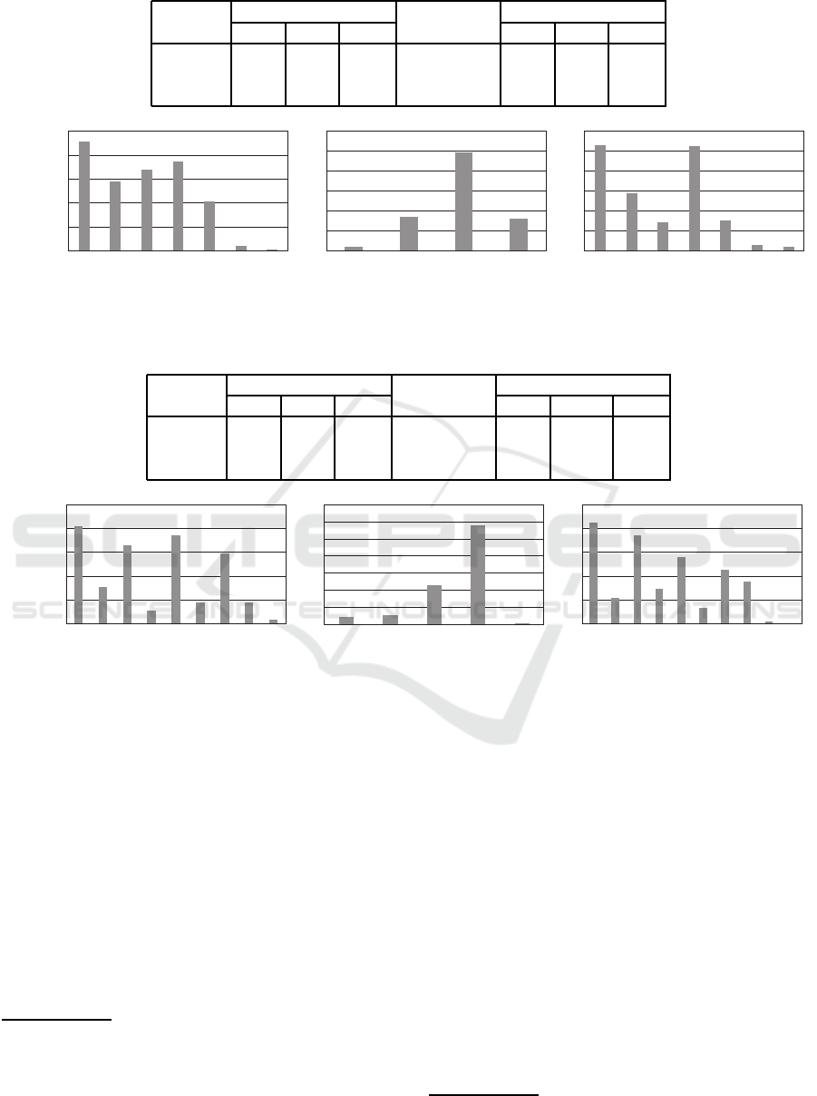
Table 1: Total cost (deterministic, 5× 5).
method individual total cost Theil index policy length
min. ave. max. min. ave. max.
sum 0.09 1.79 3.50 1.67 5 6.47 8
lxm 1.05 1.94 2.62 0.30 6 7.30 9
sumlxm 0.03 1.79 3.62 1.94 5 6.52 8
0
50
100
150
200
250
0 1 2 3 4 5 6
count
cost
sum
0
100
200
300
400
500
600
0 1 2 3
count
cost
lxm
0
50
100
150
200
250
300
0 1 2 3 4 5 6
count
cost
sumlxm
Figure 3: Histogram of total costs (deterministic, 5× 5).
Table 2: Total cost (deterministic, 7× 7).
method individual total cost Theil index policy length
min. ave. max. min. ave. max.
sum 0.09 3 6.15 1.54 8 10.35 13
lxm 2.44 3.51 4.02 0.12 8 11.79 15
sumlxm 0.06 3 6.36 1.59 8 10.53 13
0
100
200
300
400
500
0 1 2 3 4 5 6 7
8
count
cost
sum
0
200
400
600
800
1000
1200
1400
1 2 3 4 5
count
cost
lxm
0
100
200
300
400
500
0 1 2 3 4 5 6 7 8
9
count
cost
sumlxm
Figure 4: Histogram of total costs (deterministic, 7× 7).
the aggressive moves of multiple hunters in ‘lxm’
might cause noise in target moves in several instances.
Figure 3 showsthe histograms of the total cost val-
ues for all the hunters and all trials. In the case of
‘sum’, many hunters did not work at all and caught
zero cost values, while several hunters caught rela-
tively large cost values. On the other hand, ‘lxm’ re-
duced the number of idle and busy hunters. In the his-
togram of ‘lxm’, all the cost values are multiples of
ten (i.e. the number of trials for each initial setting).
Namely, the histogram is identical for the same ini-
tial setting, even though any ties are randomly broken
in all action selection steps
1
. The ‘lxm’ completely
1
Note that a hunter moves close to the target with a de-
terministic tie-break rule when it selects a move. There
might be two actions (i.e. a move and a stay) of an iden-
tical cost value for the same state in a resulting Q table. We
randomly broke such ties with uniform distribution in action
maintains the cost values among hunters in the de-
terministic case, while ‘sum’ does not capture their
individual total cost values.
Table 2 and Figure 4 show the results of the 7 ×
7 world. The size of joint state-action space to be
learned is 92, 236, 816 for this problem. In the policy
selection experiment, 450 instances were evaluated.
The results resemble the case of a 5 × 5 world, while
‘sum’ shows a variety of cost values due to the larger
size of the problems.
We also evaluated the cases where initial locations
of the target are limited to a part of the grid as follows.
• inside: the range of vertical/horizontal coordi-
nates of initial locations is [1, g − 2] where g is
a grid size and the range of all coordinates is
[0, g − 1].
• border: other locations except goal states.
selection steps.
ICAART 2019 - 11th International Conference on Agents and Artificial Intelligence
86

Table 3: Total cost (deterministic, 5× 5, partial results).
range method individual total cost Theil index policy length
min. ave. max. min. ave. max.
inside sum 0.01 1.75 3.84 2.01 5 6.50 7
lxm 1.11 1.89 2.44 0.18 6 7.41 8
sumlxm 0.56 1.92 3 0.83 5 6.97 8
border sum 0.13 1.8125 3.35 1.42 5 6.48 8
lxm 1 1.98 2.75 0.39 6 7.13 9
sumlxm 0.17 1.83 3.08 1.25 5 6.59 8
Table 4: Total cost (deterministic, 7× 7, partial results).
range method individual total cost Theil index policy length
min. ave. max. min. ave. max.
inside sum 0.08 3 6.29 1.61 8 10.36 12
lxm 2.20 3.48 4.04 0.17 8 11.54 15
sumlxm 0.24 3.12 5.76 1.35 7 10.32 13
border sum 0.10 3 6.00 1.45 8 10.40 13
lxm 2.75 3.55 4 0.07 9 12.16 15
sumlxm 0.30 3.14 5.30 1.16 8 10.59 12
Table 5: Total cost (deterministic, 5× 5, comparison with Tchebycheff functions).
method individual total cost Theil index policy length
min. ave. max. min. ave. max.
sum 0.09 1.79 3.50 1.67 5 6.47 8
max 1.95 2.39 2.90 0.13 6 8.05 11
lwt 0.71 1.88 2.67 0.59 5 7.16 9
lxm 1.05 1.94 2.62 0.30 6 7.30 9
Table 6: Total cost (deterministic, 7× 7, comparison with Tchebycheff functions).
method individual total cost Theil index policy length
min. ave. max. min. ave. max.
sum 0.09 3 6.15 1.54 8 10.35 13
max 3.71 4.08 4.27 0.02 8 11.81 17
lwt 2.33 3.46 4.02 0.14 8 11.48 15
lxm 2.44 3.51 4.02 0.12 8 11.79 15
Tables 3 and 4 show the results for both cases. The
relationship among results resembles the cases for all
initial locations.
In addition to the summation and leximax criteria,
we compared the results with the Tchebycheff func-
tions as follows.
• max: the Tchebycheff function.
• lwt: a variant of the augmented weighted Tcheby-
cheff function. Here we logically prioritized the
comparison of maximum cost values.
Tables 5 and 6 show the comparison with the Tcheby-
cheff functions. Although the maximum cost of ‘max’
is less than that of ‘sum’, it is greater than the results
of ‘lwt’ and ’lxm‘. It reveals that the proposed ap-
proach is an approximate heuristic. Moreover, ‘max’
does not maintain the total (average) cost value and
fairness. The low Theil index value of ‘max’ relates
to the high total cost values. The results of ‘lwt’ rela-
tively resemble the cases of ‘lxm’. However, the un-
fairness (i.e. the Theil index) of ‘lwt’ is greater than
‘lxm’, since its tie-break is based on the summation
criterion.
4.2.2 Non-deterministic Domain
Next we evaluated the non-deterministic process for
a 5 × 5 world. We updated all the Q-vectors, simi-
lar to the case of the deterministic process. Since the
computation is statistic and does not converge, the it-
erations of the whole updates for all the Q-vectors was
terminated at the tenth iteration. We set learning rate
α to 1, 0.5, 0.25, 0.125 and fixed discount rate γ to one,
as shown in Section 3.3.
A Study of Joint Policies Considering Bottlenecks and Fairness
87

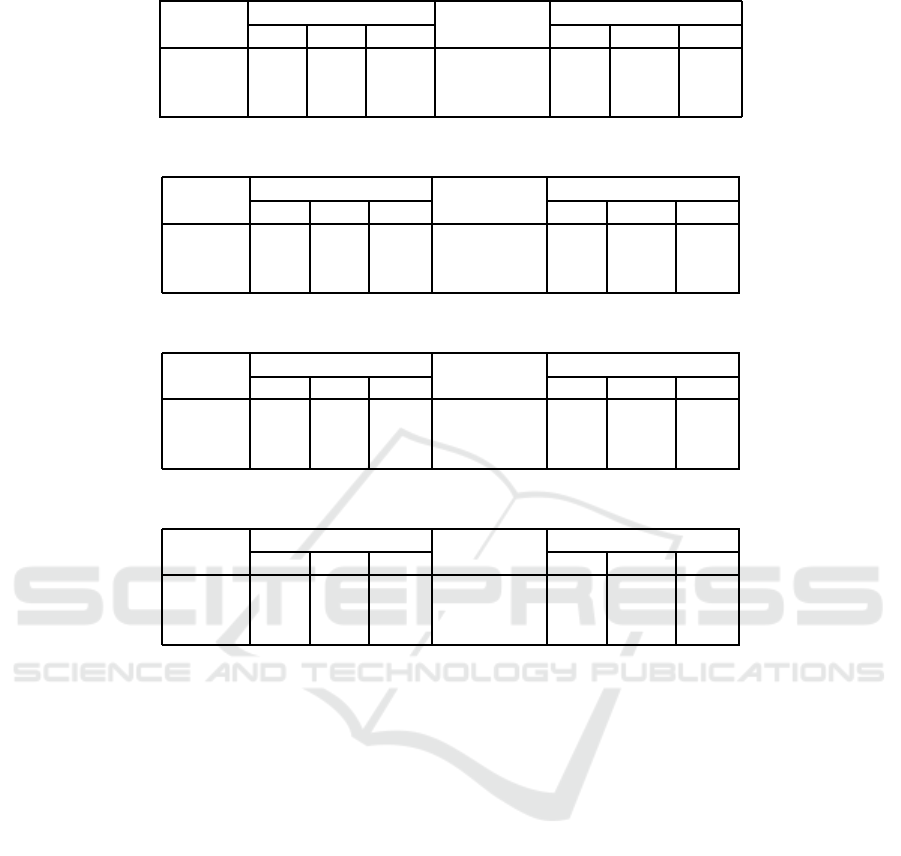
Table 7: Total cost (non-deterministic, 5× 5, α = 1).
method individual total cost Theil index policy length
min. ave. max. min. ave. max.
sum 2.54 5.94 10.43 0.85 5 22.99 110
lxm 4.38 6.72 9.04 0.35 5 23.94 102
sumlxm 4.81 7.22 9.65 0.25 5 24.86 86
Table 8: Total cost (non-deterministic, 5× 5, α = 0.5).
method individual total cost Theil index policy length
min. ave. max. min. ave. max.
sum 1.48 3.67 6.10 0.81 5 12.59 55
lxm 3.19 4.57 5.88 0.16 5 12.40 40
sumlxm 3.58 5.1 6.80 0.21 4 14.12 60
Table 9: Total cost (non-deterministic, 5× 5, α = 0.25).
method individual total cost Theil index policy length
min. ave. max. min. ave. max.
sum 0.95 3.09 5.73 1.13 5 10.39 33
lxm 2.91 4.20 5.45 0.16 4 10.26 33
sumlxm 3.31 4.76 6.37 0.22 4 12.72 49
Table 10: Total cost (non-deterministic, 5× 5, α = 0.125).
method individual total cost Theil index policy length
min. ave. max. min. ave. max.
sum 0.98 3.10 5.58 1.05 5 10.19 23
lxm 2.77 3.89 4.93 0.15 5 9.19 32
sumlxm 3.03 4.58 6.15 0.23 4 12.6 45
Tables 7-10 show the total cost values for dif-
ferent methods and learning rates. The comparison
among the methods resembles that of the determinis-
tic case, although there is the influence of stochastic
target moves. However, we found that matching the
selected actions is difficult in this case. For example,
in many aspects, the result of the different action se-
lection method for ‘lxm’ with the Euclidean distance
between (c
−
+ Q(s, a
′
)) and Q(s
−
, a
−
), or with the
leximax for the vectors of the absolute values in dif-
ference (c
−
+Q(s, a
′
))− Q(s
−
, a
−
), was often worse
than ‘sum’.
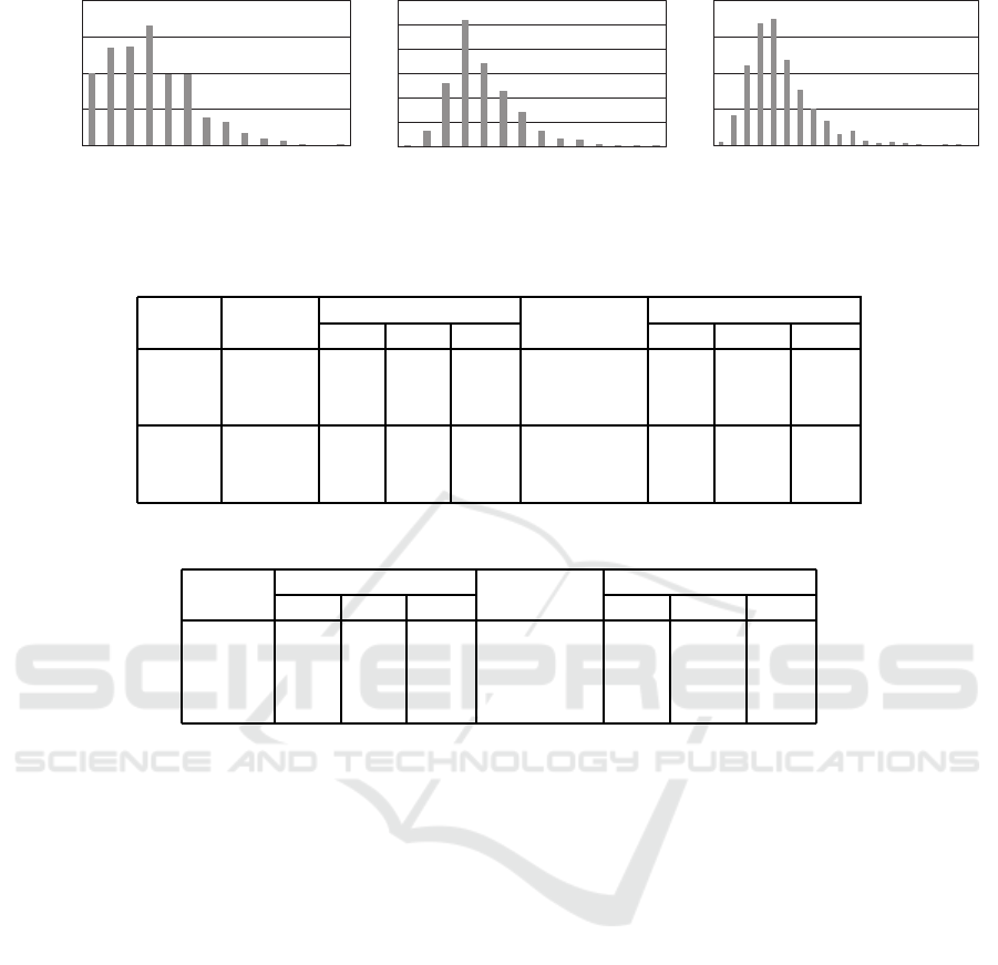
Figure 5 showsthe histograms of the total cost val-
ues for all the hunters over all the instances in the
case of α = 0.125. Although the average maximum
cost value of ‘lxm’ is less than ‘sum’ as shown in Ta-
ble 10, the histogram shows that the maximum cost
of ‘lxm’ for all the instances exceeds that of ‘sum’. In
addition, the cost values of ‘lxm’ are distributed in a
wider and higher range than the deterministic case, re-
vealing the difficulty of capturing the maximum cost
value in inexact computations.
Table 11 shows the results for different initial lo-
cations of the target. It resembles the determinis-
tic cases. Table 12 shows the comparison with the
Tchebycheff functions. In this experiment we re-
placed all leximax operators by ‘max’/‘lwt’ includ-
ing the ones to estimate compatible actions in Sec-
tion 3.3. While the results totally resemble the deter-
ministic cases, the cost values of ‘lwt’ are relatively
better than others. It is considered that the combina-
tion of maximization and summation relatively well
worked in this case. However, ‘lxm’ still reduced the
unfairness of cost values.
5 DISCUSSIONS
In this work, we employed leximax as a fundamental
criterion for fairness. Although the leximin/leximax
based approach requires more computational cost
than the conventional operation, our primary interest
is how different criteria affect joint actions. Efficient
methods that reduce computational overheadsmust be
addressed in practical domains. To reduce computa-
tional overheads, other criteria without sorted vectors
might be employed, such as the augmented weighted
Tchebycheff function, which is an extension of max-
ICAART 2019 - 11th International Conference on Agents and Artificial Intelligence
88

0
50
100
150
200
0 1 2 3 4 5 6 7 8 9 10 12 13
14
count
cost
sum
0
50
100
150
200
250
300
0 1 2 3 4 5 6 7 8 9 10 11 13
15
count
cost
lxm
0
50
100
150
200
0 2 4 6 8 10 12 14 16 18
count
cost
sumlxm
Figure 5: Histogram of total costs (non-deterministic, 5× 5, α = 0.125).
Table 11: Total cost (non-deterministic, 5× 5, α = 0.125, partial results).
range method individual total cost Theil index policy length
min. ave. max. min. ave. max.
inside sum 0.83 2.93 5.44 1.17 6 9.24 25
lxm 2.77 3.91 4.94 0.14 6 9.37 22
sumlxm 2.98 4.46 6.08 0.22 6 12.08 35
border sum 0.91 2.99 5.41 1.11 5 10.08 35
lxm 2.67 3.78 4.82 0.15 5 8.79 22
sumlxm 2.88 4.53 6.26 0.25 4 12.33 33
Table 12: Total cost (non-deterministic, 5× 5, α = 0.125, comparison with Tchebycheff functions).
method individual total cost Theil index policy length
min. ave. max. min. ave. max.
sum 0.98 3.10 5.58 1.05 5 10.19 23
max 2.83 3.90 4.98 0.15 4 9.35 39
lwt 2.7 3.75 4.77 0.16 4 8.90 21
lxm 2.77 3.89 4.93 0.15 5 9.19 32
imum scalarization where the ties are broken by the
summation. However, it only improves the worst-case
and the total cost.
Since we focused on the costs for pairs of joint
state and joint action that require a huge state-action
space, we had to employ simplified actions even
in small scale problems. To handle more types of
actions, approximate decompositions of state-action
spaces to multiple agents or partial observation are
necessary. These modifications will decrease the ac-
curacy of the proposed approach, and additional tech-
niques are necessary.
We investigated how fairness is mapped into joint
state-action space with multiple objectives. On the
other hand, action shaping is a promising technique
to reactively maintain the fairness. Indeed, our pro-
posed method partially employs an action shaping ap-
proach, since it tries to match corresponding actions.
In cases with more stochastic processes with noise,
the proposed approach will be ineffective, and reac-
tive approach will be the only solution. Although the
rotation of roles among agents is a simple solution
to distribute unfairness, we did not focus on this ap-
proach.
The proposed approach is heuristic and depends
on some kind of freeness of the problem to greed-
ily construct fair policies. In the cases where such
a greedy approach does not meet, the solution quality
of the proposed method will be decreased.
Exploration strategies for leximax might not be
straightforward. In general cases of criteria based on
minimax, the minimization operation emphasizes the
minimum-maximum cost value. Therefore, the best
first exploration based on lower bound vectors might
fall into a kind of cyclic path that resembles negative
cycles in path-finding problems.
We did not address multiple policy learning, since
its space complexity is impractical for joint state-
actions. On the other hand, if state-actions are ap-
proximately decomposed, multiple policies might be
addressed.
The proposed approach employs a single joint
state/action space and addresses bottlenecks and fair-
ness among agents. A major class of related solution
methods is the approach to converge equilibria (Hu
and Wellman, 2003; Hu et al., 2015; Awheda and
Schwartz, 2016). The comparison with equilibrium
based methods with shared and individual learning ta-
bles will be a future work.
A Study of Joint Policies Considering Bottlenecks and Fairness
89

6 CONCLUSIONS
We addressed single-policy multi-objectivereinforce-
ment learning with leximax to improve bottlenecks
and fairness among agents. We first investigated our
proposed approach for the deterministic process and
then extended it to the non-deterministic case. Our
initial results with a pursuit-problem domain show
that the learning and the action selection worked rea-
sonably well. On the other hand, the noise in the de-
cision process reduced its efficiency.
Our future work will include theoretical analysis,
more detailed evaluations in various problem domains
with some noise and partial observations, and the ex-
ploration strategies for on-line learning. The integra-
tion of reactive action shaping methods using the his-
tory of performed actions, and the investigation of ap-
proximate decompositions of joint state-action spaces
to multiple agents will also be issues.
ACKNOWLEDGEMENTS
This work was supported in part by JSPS KAKENHI
Grant Number JP16K00301 and Tatematsu Zaidan.
REFERENCES
Awheda, M. D. and Schwartz, H. M. (2016). Exponen-
tial moving average based multiagent reinforcement
learning algorithms. Artificial Intelligence Review,
45(3):299–332.
Bouveret, S. and Lemaˆıtre, M. (2009). Computing leximin-
optimal solutions in constraint networks. Artificial In-
telligence, 173(2):343–364.
Greco, G. and Scarcello, F. (2013). Constraint satisfac-
tion and fair multi-objective optimization problems:
Foundations, complexity, and islands of tractability.
In Proc. 23rd International Joint Conference on Arti-
ficial Intelligence, pages 545–551.
Hu, J. and Wellman, M. P. (2003). Nash q-learning for
general-sum stochastic games. J. Mach. Learn. Res.,
4:1039–1069.
Hu, Y., Gao, Y., and An, B. (2015). Multiagent reinforce-
ment learning with unshared value functions. IEEE
Transactions on Cybernetics, 45(4):647–662.
Liu, C., Xu, X., and Hu, D. (2015). Multiobjective rein-
forcement learning: A comprehensive overview. IEEE
Transactions on Systems, Man, and Cybernetics: Sys-
tems, 45(3):385–398.
Marler, R. T. and Arora, J. S. (2004). Survey of
multi-objective optimization methods for engineer-
ing. Structural and Multidisciplinary Optimization,
26:369–395.
Matsui, T., Matsuo, H., Silaghi, M., Hirayama, K., and
Yokoo, M. (2018a). Leximin asymmetric multiple
objective distributed constraint optimization problem.
Computational Intelligence, 34(1):49–84.
Matsui, T., Silaghi, M., Hirayama, K., Yokoo, M., and Mat-
suo, H. (2018b). Study of route optimization consid-
ering bottlenecks and fairness among partial paths. In
Proceedings of the 10th International Conference on
Agents and Artificial Intelligence, ICAART 2018, Vol-
ume 1, Funchal, Madeira, Portugal, January 16-18,
2018., pages 37–47.
Matsui, T., Silaghi, M., Okimoto, T., Hirayama, K., Yokoo,
M., and Matsuo, H. (2018c). Leximin multiple objec-
tive dcops on factor graphs for preferences of agents.
Fundam. Inform., 158(1-3):63–91.
Moffaert, K. V., Drugan, M. M., and Now´e, A. (2013).
Scalarized multi-objective reinforcement learning:
Novel design techniques. In 2013 IEEE Symposium on
Adaptive Dynamic Programming and Reinforcement
Learning (ADPRL), pages 191–199.
Sen, A. K. (1997). Choice, Welfare and Measurement. Har-
vard University Press.
Sutton, R. S. and Barto, A. G. (1998). Reinforcement learn-
ing : an introduction. MIT Press.
ICAART 2019 - 11th International Conference on Agents and Artificial Intelligence
90