
Oscillating Mobile Neurons with Entropic Assembling
Eugene Kagan
1,2
and Shai Yona
3
1
Department of Industrial Engineering, Ariel University, Ariel, Israel
2
LAMBDA Lab, Tel-Aviv University, Tel-Aviv, Israel
3
Department of Industrial Engineering, Ariel University, Ariel, Israel
Keywords: Neural Network, Oscillating Neurons, Mobile Neurons, Neurons Ensemble, Entropy.
Abstract: Functionality of neural networks is based on changing connectivity between the neurons. Usually, such
changes follow certain learning procedures that define which neurons are interconnected and what is the
strength of the connection. The connected neurons form the distinguished groups also known as Hebbian
ensembles that can act during long time or can disintegrate into smaller groups or even into separate
neurons. In the paper, we consider the mechanism of assembling / disassembling of the groups of neurons.
In contrast to the traditional approaches, we set ourselves to “the neuron’s point of view” and assume that
the neuron chooses the neuron to connect with following the difference between the current individual
entropy and the expected entropy of the ensemble. The states of the neurons are defined by the well-known
Hodgkin-Huxley model and the entropy of the neuron and the neuron’s ensemble is calculated using the
Klimontovich method. The suggested model is illustrated by numerical simulations that demonstrate its
close relation with the known self-organizing systems and the dynamical models of the brain activity.
1 INTRODUCTION
Artificial neural networks are mathematical models
of nervous systems of living organisms. Formally,
such networks are the systems of interconnected
basic elements – neurons, and their functionality
depends on changing connectivity between the
neurons. The neurons act according to the activation
function and send the output signals with respect to
the sum of input signals.
In the traditional considerations of artificial
neural networks (Fausett, 1995), (Russell and Norvig,
2010), connectivity between the neurons is defined
by certain learning procedures that specify which
neurons are interconnected and what is the strength
of the connection. Then, the neurons change their
states with respect to the sum of the input signals.
The output signals are transmitted with respect to the
states of the neurons, and after transmitting the
outputs the neurons return to their initial states.
In the other approaches mainly used in
synergetics (Haken, 2008), the changes of the
neurons’ states are directly considered as oscillations
with varying period near a neutral state (Kuzmina,
Manykin and Grichuk, 2014). The variations of the
period in each neuron depend on the oscillations of
the neighbouring neurons. This point of view
introduces neural networks into general framework
of dynamical systems (Zaslavsky, 2007) and allows
their studies using the methods of non-linear
dynamics and statistical physics (Klimontovich,
1991). The connectivity between the neurons in such
dynamical oscillating systems is defined from “the
neuron’s point of view”, where each neuron
independently chooses with which neuron it prefers
to connect.
Then, there arises a natural question: what
factors lead the neurons to connect one with the
other and to form the ensembles and what factors
lead the neurons to disconnect and to disassemble
the existing ensembles?
The popular Hebbian theory (Hebb, 1949)
presents the reasons of such choice in the qualitative
form and specifies the connection between the
neurons in the terns of sparking synchronization; a
brief overview of the Hebbian theory and its
successors was published by Fregnac (Fregnac,
2003); one of the attempts of mathematical
formalization of this theory in the terms of
dynamical systems was conducted by Gerstner and
Kistler (Gerstner and Kistler, 2002).
In the paper, we present the model of assembling
/ disassembling of the groups of neurons. Following
260
Kagan, E. and Yona, S.
Oscillating Mobile Neurons with Entropic Assembling.
DOI: 10.5220/0007571202600266
In Proceedings of the 11th International Conference on Agents and Artificial Intelligence (ICAART 2019), pages 260-266
ISBN: 978-989-758-350-6
Copyright
c
2019 by SCITEPRESS – Science and Technology Publications, Lda. All rights reserved

the dynamical systems’ approach, we set ourselves
to “the neuron’s point of view” and assume that the
neuron chooses the neuron to connect with following
the difference between the current individual
entropy and the expected entropy of the ensemble.
The states of the neurons are defined by the
simple model of the sparking neurons developed by
Izhikevich (Izhikevich, 2003, Izhikevich, 2007) on
the basis of the well-known equations by Hodgkin
and Huxley (see e.g. (Sterratt, Graham, Gillies and
Willshaw, 2011)). The entropy of the neuron and the
neuron’s ensemble is calculated using the
Klimontovich method (Klimontovich, 1987),
(Klimontovich, 1991).
The suggested model is illustrated by direct
numerical simulations that demonstrate its close
relation with the Turing system (Turing, 1952),
(Leppanen, 2004) and the other models of self-
organizing systems.
2 GENERAL DESCRIPTION OF
THE MODEL
The suggested model is based on the distributed
dynamical system widely known as oscillating
active media (Mikhailov, 1990). In this media, each
element is considered as an oscillator (linear or non-
linear) interconnected with the other elements. As a
result, over the media appear the ordered wave
structures created by the synchronized and
desynchronized oscillations of the elements.
In the model, we consider the neurons as
oscillators that can be (or can be not) connected with
the other neurons. The interconnected neurons form
ensembles that act as oscillating systems, and
separate neurons act as point-like oscillators. The
last assumption contrasts with the usual assumption
applied to artificial neural networks, where each
neuron spikes with respect to the input signals
received from the other neurons and does not spike
without such inputs. The scheme of the considered
network is shown in Figure 1.
Figure 1: The scheme of the network with oscillating
neurons.
Notice that similar networks already appeared in the
studies of the Gorkiy physical school, especially in
the works by Vedenov et al. (see e.g. Vedenov, Ejov
and Levchenko, 1987)); the contemporary
developments in this direction are published in the
book by Kuzmina et al. (Kuzmina, Manykin and
Grichuk, 2014).
The main question that arises in the studies of
the networks of autonomous oscillating neurons is:
- what factors lead the neuron to connect with one
neuron and to avoid connection with the other
neuron?
In the other words,
- what factors lead neurons to assemble and to
disassemble?
In the suggested model, we assume that the
neurons’ interconnections are defined by the
difference between the entropies of the separate
neurons and the entropies of the neurons’ ensembles.
The process of connecting and disconnecting is the
following.
Consider two oscillating neurons and . The
equations of their dynamics allow calculation of the
entropies
and
of the neurons and the entropy
of the coupled oscillator that consists of
the neurons and . We postulate that the neurons
and create connection between them if
and
(1a)
or
and
(1b)
Once been interconnected, the neurons act in pair
that can create connections with the other neurons
following the same entropic criterion. At the
moment when the entropy of the pair
reaches the
value such that the inequality (1) does not hold, the
neurons break their connection and continue acting
separately. The same reasoning is also applied to the
formation of the neuron’s ensembles that include
more than two neurons.
This model was inspired by the considerations of
the neural networks with mobile neurons (Apolloni,
Bassis, and Valerio, 2011), especially – by their
application to the mobile robots control Kagan,
Rybalov and Ziv, 2016). It does not require external
learning processes that define the strength of the
neurons’ interconnections but, in contrast, forms a
system that reacts to the inputs by changing internal
structure.
The model requires formal equations of the
neurons’ activity and corresponding methods of
entropy calculation. In the next section, we start with
the simple model of spiking neuron.
Oscillating Mobile Neurons with Entropic Assembling
261

3 THE SPIKING NEURON AND
ITS CONNECTIVITY
The considered model of the network of oscillating
neurons assumes that the output of each neuron in
the network oscillates near some stable value. The
well-known model of such oscillating neuron was
suggested by Hodgkin and Huxley who considered
the dynamics of its electric potential (see e.g.
(Sterratt, Graham, Gillies and Willshaw, 2011)).
Starting from the Hodgkin and Huxley model, in
2003 Izhikevich suggested the simpler model that is
formulated as follows (Izhikevich, 2003). Denote by
the membrane potential of the neurone and by
the membrane recovery variable that represents the
negative feedback for . Then, the spike of the
neurone is defined by the system of two equations:
,
(2a)
,
(2b)
with the reset condition
if then and .
(3)
In the equations, stands for the synaptic currents;
parameter is the time scale of the recovery;
parameter is the sensitivity of the recovery to
the fluctuations of the membrane potential; and
parameters and are the after-spike
reset values caused by fast and slow fluctuations of
the potential, respectively. In the next years, the
model (2)-(3) was intensively studied and formed a
basis for dynamical models of neural networks
(Izhikevich, 2007).
Let us rewrite the system (2) in the form of the
oscillator equation that is
,
(4)
where following the values appeared in the system
(2) , and . It is clear that
equation (4) is the equation of non-linear forced
oscillator with the feedback parameter and
external drive
.
Equation (4) has the same form as the well-
known van der Pol equation (see e.g. (Klimontovich,
1991)) and differs from it in the power of in the
“friction” coefficient: in the van der Pol equation it
is
and here it is
. Nevertheless, because of its
form and the bounds defined by the reset condition
(3) this equation is suitable for calculations of the
entropy developed for the van der Pol equation.
Now let us consider the external drive
. In
the Izhikevich model the variable is defined as a
synaptic current, or, in the other words, as a variable
that represents the flow via the neuron’s inputs and
outputs. Then, the value
in the equation (4)
stands for the changes of the input/output flow that
completely meets the Kawahara model of neural
interactions (Kawahara, 1980); but again, notice the
indicated difference between equation (4) and the
van der Pol equation.
In our model, we apply the week coupling
suggested by Rand and Holmes (Rand and Holmes,
1980) and define drive
between neuron with
the membrane potential
and neuron with the
membrane potential
as
.
(5)
In the considered version of the model, we assume
that
. As a result, the
connectivity between the neurons is defined by the
single weight parameter
that also can be
specified with respect to the entropies of the
neurons. In the next section we define these
entropies.
4 ENTROPY OF THE NEURONS
AND OF THEIR ENSEMBLES
Entropy of the neurons of their ensembles is defined
following the method suggested by Klimontovich; in
his book (Klimontovich, 1991) this approach is
considered in details. The idea of the method is as
follows.
At first, consider dynamical equation of the
system as the Langevin equation with certain source
that describes the random walk. At second, using the
Fokker-Plank equation, obtain the probability
distribution of locations and velocities of the
walking particles. Finally, calculate the entropy of
this distribution (relatively to the distribution of the
source used in the Langevin equation) that is the
entropy of the considered system, in our case – of
the neuron.
In the original work, Klimontovich considered
the van der Pol equation; here we apply this method
directly to the system (4).
ICAART 2019 - 11th International Conference on Agents and Artificial Intelligence
262

For definition of the entropy of separate neuron
without interactions, we assume that
. Then,
the Langevin equation for the equation (4) has the
following form:
,
(6a)
,
(6b)
where
is the stochastic source that is the
Gaussian noise and is the intensity of the source.
The term
is a friction coefficient that
defines dissipation forces and the term
represents potential field that depends on the state of
the system.
For this equation, the Fokker-Plan equation of
the dynamics of distribution
in the phase
space
is
.
(7)
Because of the reset condition (3) it is rather
problematic to find analytic solution of this
equation. Nevertheless, it can be shown that it has
the Gauss-like form:
,
(8)
where strictly positive function depends also on
the parameter and positive function depends on
the parameters , and (see equation (4)). In
addition, it is assumed that
.
Finally, the entropy
of the neuron with the
steady state distribution
is
,
(9)
where plays a role of the Boltzmann
coefficient.
The entropy of the ensemble of the neurons is
defined using the external drive
of the neuron
by the members of its ensemble. In the case of a pair
of neurons, it is defined by the equation (5). The
Fokker-Plank equation for the distribution
of the neuron acting in pair with the
neuron is
.
(10)
Then, the entropy
of the neuron biased by the
neuron is
.
(11)
where
is a steady state distribution over the
velocities of the neurons and . The entropy
of the neuron biased by the neuron is defined by
the same manner. Another method (Klimontovich,
1991) of defining the entropies
and
is to
use the Kullback-Leibler entropy.
Finally, entropy of the neurons ensemble of
neurons (Klimontovich, 1991) is obtained using the
average distribution
that represents the distribution
of the average velocities
of randomly moving (but
not necessary Brownian) particles. Such distribution
is governed by the Turing system (Turing, 1952),
(Leppanen, 2004) of the form
,
(12a)
,
(12b)
where function
stands for the activator function
and auxiliary function stands for the inhibitor
function, and the functions and specify the
positive and negative feedback, respectively.
Then the entropy of the ensemble is
.
(13)
These formulas are widely used in statistical
physics for description of the behaviour of
elementary particles, but for the description of the
activity of neural network the idea to use the average
coordinates and velocities seems to be not the best
one. More realistic method can be based on the
distribution of active and non-active neurons as it is
defined by the methods of population dynamics see
e.g. (Kagan, Ben-Gal, 2015).
Oscillating Mobile Neurons with Entropic Assembling
263
5 NUMERICAL SIMULATIONS
Numerical simulations illustrate activity of the
neurons. For the simulations, we directly apply the
simple numerical schemes to the equations presented
in the previous section.
In all simulations, parameters have the values
indicated in the previous section that are: ,
, and . These values appear
in the original paper by Izhikevich (Izhikevich,
2003). In the other equations we used the parameters
, , ,
,
and
. In order to obtain clear illustration of the
neuron activity, the value of the frequency
was chosen with respect to the time interval
.
Let us consider the activity of the single neuron.
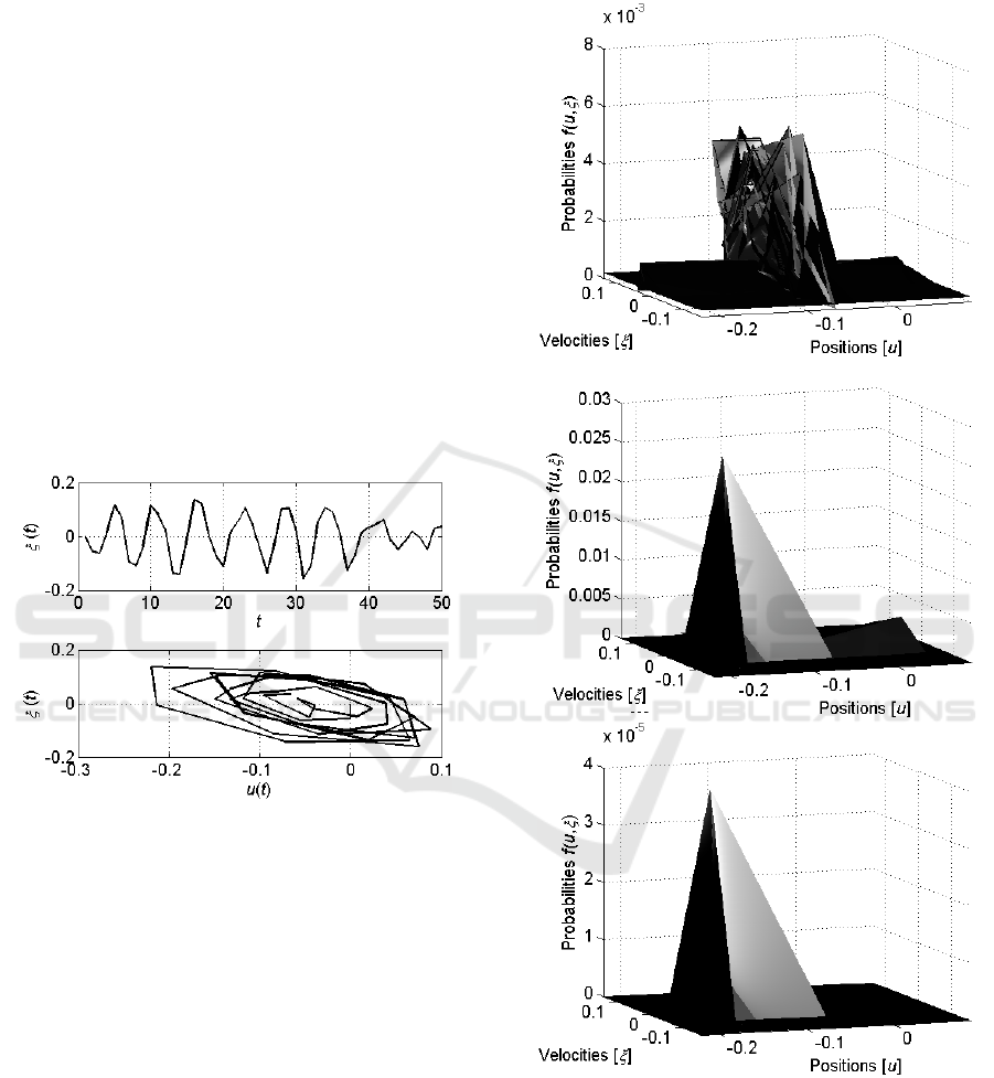
Figure 2 shows the graph of the velocity
and
the phase portrait of the neuron defined by the
Langevin equation (6).
Figure 2: The graph of the velocity and the phase portrait
of a single neuron described by the Langevin equation (6).
It is seen that the neuron demonstrates the oscillating
behaviour with certain randomness.
The next Figure 3 shows evolution of the
distribution
in time starting from the
uniform distribution.
Evolution of the entropy
starting from the
last stages of its decreasing is shown in Figure 4.
As it was expected, the entropy starts with the
maximal value that corresponds to the uniform
distribution and exponentially decreases to some
small value and then oscillates near this value.
Now, let us consider activity of the pair of
neurons described by the Fokker-Plank equation
(10). The first neuron in the pair is the neuron
considered in the previous simulations and the
second neuron is defined by the same equations with
the same values of the parameters. The difference
between the neurons caused by randomness of the
values generated by the stochastic sources
.
Figure 3: Evolution of the distribution
for a
single neuron as it is defined by the Fokker-Plank equation
(7) from the initial uniform distribution. The first graph
shows the distribution
at the starting stages,
; the second – at the middle, , and the last – at the
end, , of the trial.
ICAART 2019 - 11th International Conference on Agents and Artificial Intelligence
264
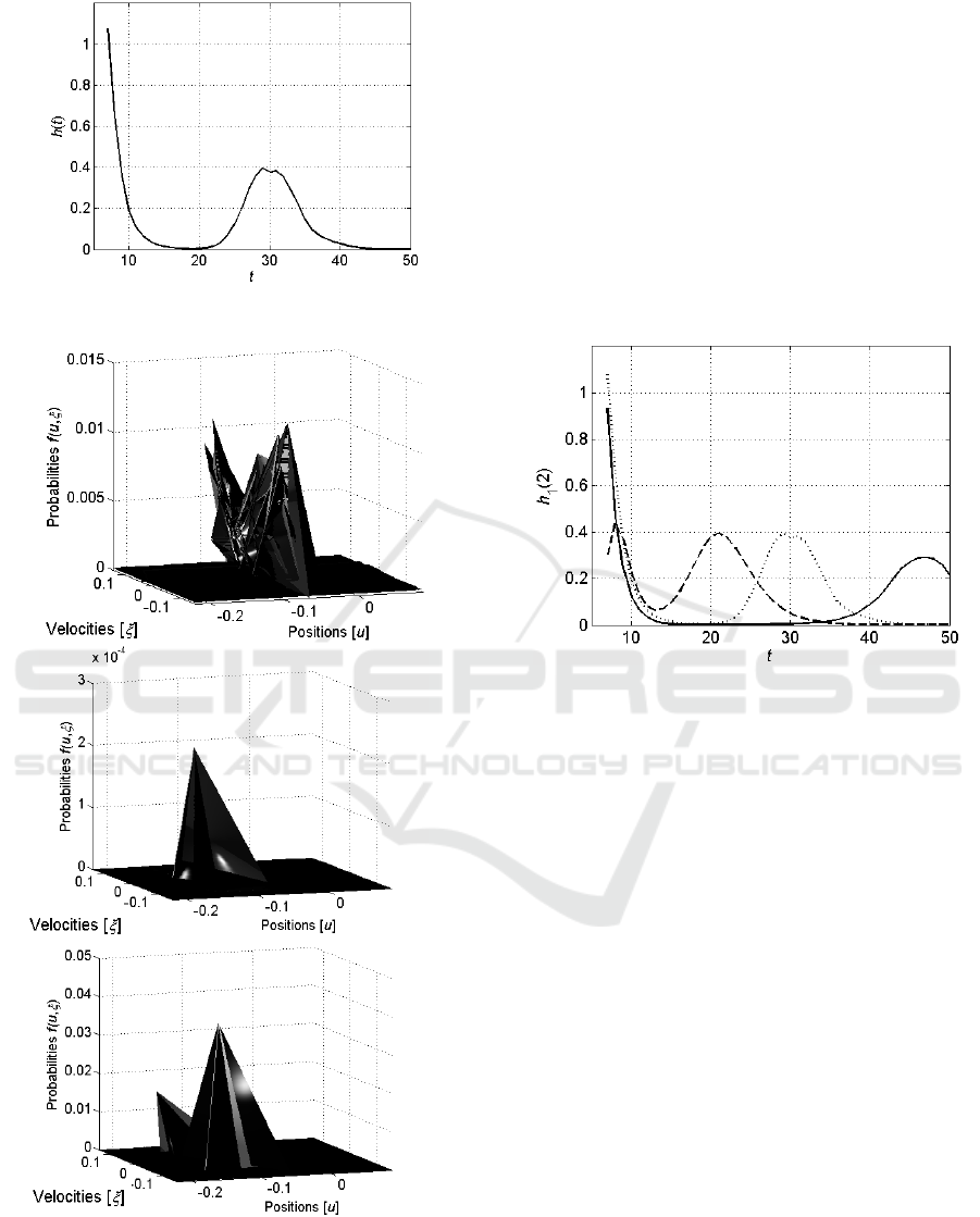
Figure 4: Evolution of the entropy
of a single neuron.
Figure 5: Evolution of the distribution
of
neuron acting in pair with neuron as it is defined by
the Fokker-Plank equation (10). The first graph shows the
distribution
at the starting stages, ; the
second – at the middle, , and the last – at the end,
.
Evolution of the distribution
of
neuron acting in pair with neuron is shown in
Figure 5. It is seen that this evolution is similar to
the evolution of the distribution
of single
neuron.
The entropies
and
of the neurons
and acting separately exponentially decrease and
oscillate near some small value, and the same holds
with the entropy
of the neuron biased by the
neuron . However, the velocity of decreasing and
the frequency of oscillations are different.
Figure 6 shows the last stages of the decreasing
of these three entropies and their oscillations.
Figure 6: Last stages of the decreasing of the entropies
(dotted curve) and
(dashed curve) of the
neurons and , respectively, and of the entropy
(solid curve) of the neuron biased by the neuron .
It is seen that starting from the time , while
, both
and
.
Hence, following the suggested model of creating
connections between the neuron’s (see Section 2,
especially – inequalities (1)), the neurons and
will interconnect and start acting in pair.
However, at the time the entropy
of the pair of neurons becomes greater than the
entropies
and
of each of the neurons
acting separately. Then, the neurons disconnect and
begin to act separately.
As indicated above, the neurons ensembles that
include more than two agents act in the same
manner, but the entropy of the ensemble should be
calculated by the other methods, for example, using
the models population dynamics see e.g. (Kagan,
Ben-Gal, 2015).
Oscillating Mobile Neurons with Entropic Assembling
265

6 CONCLUSIONS
The considered neural network consists of the
oscillating mobile neurons that connect and
disconnect with respect to their entropies and the
entropy of the ensemble. The states of the neurons
are defined on the basis of the well-known Hodgkin-
Huxley model that defines the oscillations of the
neurons’ activity.
Such definition allows calculation of the entropy
of the neuron and the neuron’s ensemble using the
Klimontovich method that is widely used in
statistical physics.
The suggested approach contrasts with the
traditional methods, where the connections between
the neurons are governed by the external learning
procedures, and specifies the neurons’ connections
on the basis of the neurons’ internal properties.
Numerical simulations confirm feasibility of the
suggested model and demonstrate the required
properties of the entropy of separate neurons and of
the neurons’ ensembles. In particular, it was shown
that the entropy of the single neuron periodically
obtains the values greater than the values of the
entropy of this neuron acting in pair with the other
neuron. Following the suggested model, connection
and disconnection of the neurons is governed by this
inequality.
The suggested mechanism of assembling /
disassembling is equal to motion of the neurons
toward the other neurons or away from them,
respectively, and the information about the neurons’
entropies is transmitted via the glia.
REFERENCES
Apolloni, B., Bassis, S., Valerio, L., 2011. Training a
network of mobile neurons. In Proc. Int. Joint Conf.
on Neural Networks, San Jose, CA, 1683-1691.
Fausett, L., 1994. Fundamentals of Neural Networks:
Architectures, Algorithms and Applications. Upper
Saddle River, NJ, Prentice Hall.
Fregnac, Y., 2003. Hebbian cell assembles. In
Encyclopaedia of Cognitive Science, Nature
Publishing Group, 320-329.
Gerstner, W., Kistler, W., 2002. Mathematical
formulations of Hebbian learning. Biological
Cybernetics, 87, 404-415.
Haken, H., 2008. Brain Dynamics. An Introduction to
Models and Simulations. Springer-Verlag,
Berlin/Heidelberg, 2
nd
edition.
Hebb, D. O., 1949. The Organization of Behaviour: A
Neuropsycological Theory. Wiley & Sons, New York.
Izhikevich, E., 2003. Simple model of spiking neurons.
IEEE Trans. Neural Networks, 14, 1569-1572.
Izhikevich, E., 2007. Dynamical Systems in
Neuroschience: The Geometry of Excitability and
Bursting. The MIT Press, Cambridge, MA, London,
UK.
Kagan, E., Ben-Gal, I., 2015. Search and Foraging.
Individual Motion and Swarm Dynamics. CRC Press /
Chapman & Hall / Taylor & Francis, Boca Raton, FL,
Kagan, E., Rybalov, A., Ziv, H., 2016. Uninorm-based
neural network and its application for control of
mobile robots. In Proc. IEEE Int. Conf. Science of
Electrical Engineering, Eilat, Israel.
Kawahara, T., 1980. Coupled van der Pol oscillators – a
model of excitatory and inhibitory neural interactions.
Biological Cybernetics, 39(1), 37-43.
Klimontovich, Yu., 1987. Entropy evolution in self-
organization processes: H-theorem and S-theorem.
Physica, 142A, 390-404.
Klimontovich, Yu., 1991. Turbulent Motion and the
Structure of Chaos. Springer Science + Business
Media, Dordrecht.
Kuzmina, M., Manykin, E., Grichuk, E., 2014. Oscillatory
Neural Networks. De Gruyter, Berlin/Boston.
Leppanen, T., 2004 Computational Studies of Pattern
Formation in Turing Systems. Helsinki University of
Technology, Laboratory of Computational
Engineering, Report B40, Helsinki.
Mikhailov, A. 1990. Foundations of Synergetics I.
Distributed Active Systems. Springer-Verlag, Berlin,
2
nd
edition.
Rand, R., Holmes, P., 1980. Bifurcation of periodic
motions in two weakly coupled van der Pol oscillators.
Int. J. Non-Linear Mechanics, 15, 387–399.
Russell, S., Norvig, P., 2010. Artificial Intelligence. A
Modern Approach. Pearson Education, Upper Saddle
River, NJ, 3
rd
edition.
Sterratt, D., Graham, B., Gillies, A., Willshaw, D., 2011.
Principles of Computational Modelling in
Neuroscience. Cambridge University Press,
Cambridge, MA.
Turing, A., 1952. The chemical basis of morphogenesis.
Phil. Trans. Royal Soc. London, B, Biological
Sciences, 237(641), 37-72.
Vedenov, A., Ejov, A., Levchenko, E., 1987. Nonlinear
dynamical systems with memory and the functions of
neouron ensembles. In Gaponov-Grekhov A.,
Rabinovich, I (eds.) Nonlinear waves: Structures and
Bifurcations, Nauka, Moscow, 53-67 (in Russian).
Zaslavsky, G., 2007. Physics of Chaos in Hamiltonian
Systems. Imperial College Press, London, 2
nd
edition.
ICAART 2019 - 11th International Conference on Agents and Artificial Intelligence
266
