
An Agent-based Approach to a Temporal Headway Development
Statistics in Urban Traffic using Three-phase Theory
Maximilian Kumm and Michael Schreckenberg
Physics of Transport and Traffic, University of Duisburg-Essen, Lotharstr. 1, 47057 Duisburg, Germany
Keywords: Multi-Agent System, Automated Vehicle, Car2X, Temporal Headway Development, Three-phase Traffic
Theory, Kerner-Klenov Model, Vehicle Speed in Free Flow, Urban Traffic, Empirical Speed Distribution.
Abstract: An automated vehicle is supposed to merge into the major street of a T-intersection, while disturbing the
ongoing traffic as little as possible. At the same time, different requirements regarding its driving strategy
have to be fulfilled with respect to safety, comfort and energy conditions. It is desirable to enable a fluent
automated drive and to avoid stopping during the approach at all. We implemented an agent-based simulation
using the Kerner-Klenov model in framework of the three-phase traffic theory. Using a high number of
interacting vehicles leads to a multi-agent system (MAS). A normal distributed free flow parameter based on
empirical traffic data is introduced and serves as an input parameter to the simulations. The simulations output
yield temporal headway development-statistics, which enables a prediction of the traffic situation on the major
street. This allows the automated vehicle to adjust its speed in preparation of merging into the best possible
gap considering the above-mentioned requirements. Hence, taking these statistics into account helps to
optimise the driving strategy of the automated vehicle.
1 INTRODUCTION
Automated vehicles are expected to play a major role
in road traffic within the next decades. Thus, it is
necessary to manage the oncoming heterogeneous
traffic between classical and automated vehicles.
Especially human behaviour represents a factor of
uncertainty in this context. That is why we choose a
statistical approach to make different driving
behaviour as predictable as possible.
This work describes an approach that allows
automated vehicles to interact with common road
traffic in a safe and efficient way.
At first, an overview is given about the most
important theories and agent-based models which are
used to describe road traffic (subsection 1.1 to 1.3).
Finally, subsection 1.4 describes the specific
application.
1.1 Nagel-Schreckenberg Model
In 1992 Kai Nagel and Michael Schreckenberg came
up with the idea of using cellular automata (CA) to
simulate freeway traffic (Nagel and Schreckenberg,
1992). Using this microscopic approach, they were
able to model a phase transition from laminar flow to
congested traffic with increasing vehicle density.
Hence, the Nagel-Schreckenberg model
distinguishes two phases of traffic (Kerner, 2017).
Several advancements of the model were suggested
since then; to name just a few: (Rickert, 1996),
(Hafstein, 2004), (Chmura, 2014).
1.2 Three-phase Traffic Theory
However, in three-phase traffic theory (Kerner, 2004)
one more phase of traffic is taken into account. The
theory divides congested traffic into the synchronized
flow phase S and the wide moving jam phase J by
introducing a so-called synchronisation space gap
between consecutive vehicles.
The synchronisation space gap is a direct
consequence of humans accepting different distances
to the preceding vehicle as long as this gap is not
getting smaller than the safe space gap
. The safe
space gap is related to the safe speed
(Krauss et
al., 1997). Due to the associated speed adjustment, the
synchronised flow phase S is explained.
By contrast, the wide moving jam moves
downstream through any other traffic phase, while
238
Kumm, M. and Schreckenberg, M.
An Agent-based Approach to a Temporal Headway Development Statistics in Urban Traffic using Three-phase Theory.
DOI: 10.5220/0007484602380243
In Proceedings of the 11th International Conference on Agents and Artificial Intelligence (ICAART 2019), pages 238-243
ISBN: 978-989-758-350-6
Copyright
c
2019 by SCITEPRESS – Science and Technology Publications, Lda. All rights reserved

maintaining its downstream front’s mean velocity.
This is the characteristic feature of phase J.
Last but not least, there is the non-congested
traffic phase, which is called the free flow traffic
phase F. It usually occurs when there is a low traffic
density, i.e. when interactions between single
vehicles are negligible. Consequently, they are free to
choose their speed as long as it is in conformity with
underlying road limitations like speed limits.
Usually, through an increase in density, e.g. at a
bottleneck (Kerner, 2000), a phase transition from
free flow F to synchronized flow S can occur.
The classical flow instability (Chandler and
Herman, 1958) has been taken over by the three-
phase traffic theory. Within Kerner’s Theory, it is
responsible for the spontaneous emergence of wide
moving jams leading to a phase transition from S to J.
1.3 Kerner-Klenov Model
The related microscopic and stochastic model version
of the three-phase traffic theory is known as Kerner-
Klenov model. Single vehicles are supposed to be the
simulation’s agents. Due to the high number of
interacting vehicles, it is a multi-agent system (MAS).
In this work, we use the model version that is discrete
in space and time (Kerner and Klenov, 2009). All
containing parameters and functions are adapted to
urban traffic (Kerner, 2013). Although this model is
not cellular automaton-based, some of its behaviour
is quite similar to (Nagel and Schreckenberg, 1992).
In addition, the used assumptions are based on
empirical traffic data. As it is shown in Chapter 1, 2
and 4 in (Kerner, 2017), the model’s underlying
three-phase traffic theory is best suited to describe
traffic.
For a detailed view on the underlying
mathematics and the high complexity of the model,
please see (Kerner, 2017).
The spatial headway
of a vehicle for time step
n is defined as follows (Kerner, 2017):
(1)
where
is the position of the vehicle,
the
position of its preceding vehicle and the vehicle
length including the mean space gap between vehicles
that are in standstill. Furthermore, the temporal
headway
is obtained by dividing equation (1) by
the vehicle speed
:
(2)
The time step of the simulation is always marked
by the index .
As mentioned above, vehicles being in the free
flow traffic phase F are capable of choosing their
speed largely free. The related parameter within the
Kerner-Klenov model is called
.
1.4 Application
Usually, the Kerner-Klenov model is applied to
analyse macroscopic properties like phase transitions
at bottlenecks. The predictions made by the three-
phase traffic theory are matching empirically
observed traffic patterns (Kerner, 2017, pp. 73-81).
However, the present case is about a microscopic
analysis of vehicle headway development and brings
a new application to the model.
Figure 1: T-intersection with common road traffic on its
major street (yellow boxes). An automated vehicle (red
box) is approaching from below and tries to merge into the
ongoing traffic (purple marked headway). The question is
how the marked headway has developed, when reaching the
intersection point
. There is a speed limit of 30 km/h.
Within one realisation, all containing vehicles are initialised
at
using the same temporal headway
.
The specific application contains a T-intersection
(figure 1) without traffic lights but high numbers of
common vehicles. An automated vehicle (red box) is
approaching the intersection point aiming at merging
into the ongoing traffic (yellow boxes). When the
current traffic situation on the major street is provided
to the automated vehicle, a statistical analysis based
algorithm can predict the best gap for merging into
the street. In terms of safety, comfort and energy
conditions, the approach to the intersection should not
be interrupted by a stop. That is why, it is necessary
to carry out a statistical analysis of how the headway
between two consecutive vehicles on the major street
develops, first.
Following this guideline, we implemented a
simulation based on the Kerner-Klenov model
An Agent-based Approach to a Temporal Headway Development Statistics in Urban Traffic using Three-phase Theory
239
adapted to urban traffic using open boundary
conditions. Within one simulation, all containing,
identical vehicles were initialised at
with the same
initial temporal headway
. Different simulations -
with thousands of cars each - were realised by using
the following values:
(3)
When the middle of the marked space gap in
figure 1 reaches the intersection point
, the
temporal headway is buffered. Whenever this
condition is met, we call the set of the corresponding
time steps
. Doing so with a large number of cars
enables a statistical evaluation. The related temporal
headway
is called
(4)
In this work, we choose the distance
between
the point, where the cars are initialised
and the
intersection point
as 100 meters.
(5)
The publically funded project “MEC-View” aims
at collecting vehicle data from an urban major street
using an infrastructure-based sensor system. Like in
this work, the sensor system monitors approximately
100 meters of the major street. That is why this value
is used for the parameter
. The collected data is
provided to an automated vehicle approaching the
concerned T-intersection. Using this information
supports the automated vehicle to merge into the
ongoing traffic.
2 RESULTS
2.1 Constant Free Flow Parameter
To our best knowledge, the Kerner-Klenov model is
always used with a constant free flow parameter. This
means in particular, that the same free flow speed
is assigned to all vehicles. Due to the speed limit
on the current T-intersection, it is set to 30 km/h.
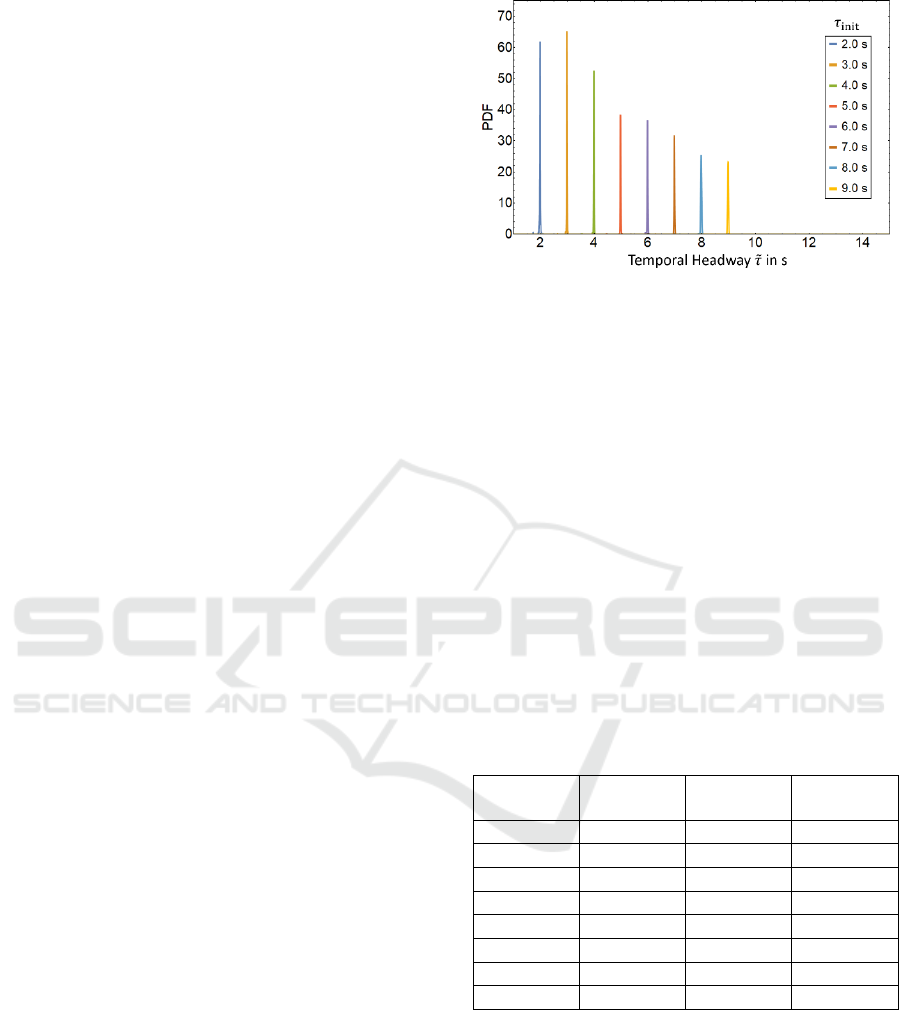
In figure 2, the concerning results are shown for
the usual case (
= const.). Sharp peaks are
resulting for the PDF, which reflects the temporal
headway distribution. That means seems to stay
practically constant within the distance
and is not changing significantly. Thus, for the initial
temporal headway applies:
Figure 2: Probability density function (PDF) against the
temporal headway at the intersection point
for
different initial temporal headways
. For the free flow
parameter of each vehicle applies
km/h. All
vehicles are initialised at
(see figure 1). Due to only
slight model fluctuations, sharp peaks are seen, i.e. the
temporal headway is not changing significantly within the
range from
to
(100 meters).
(6)
This fact is also confirmed by a very small
variance in combination with an almost equal mean
value (see Table 1). Because these results do not seem
to be realistic, we present a collected empirical
dataset in the following subsection 2.2 to justify a
different approach in subsection 2.3.
Table 1: Mean, variance and skewness of the distributions
shown in figure 2. Please note: due to the peak-like shape
of the underlying distributions, the variance is specified in
10
-5
s.
[s]
Mean
[s]
Variance
[10
-5
s²]
Skewness
[s³]
2.0
1.979
0.50
-3.69
3.0
2.981
0.41
-14.15
4.0
3.980
0.73
-14.75
5.0
4.979
1.33
-13.63
6.0
5.979
1.41
-14.97
7.0
6.978
1.98
-15.46
8.0
7.977
2.97
-13.94
9.0
8.997
3.57
-13.85
2.2 Free Flow Speed in Empirical
Speed Data
In order to obtain reliable vehicle speed data, we
performed a camera-based measurement on an urban
straight road in Duisburg, Germany with a speed limit
of 50 km/h. The decision for this road was made
because there is no influence on passing vehicles e.g.
through traffic lights, speed cameras or obstructed
ICAART 2019 - 11th International Conference on Agents and Artificial Intelligence
240
view. Consequently, all road users can choose an
appropriate personal speed taking into account the
speed limit.
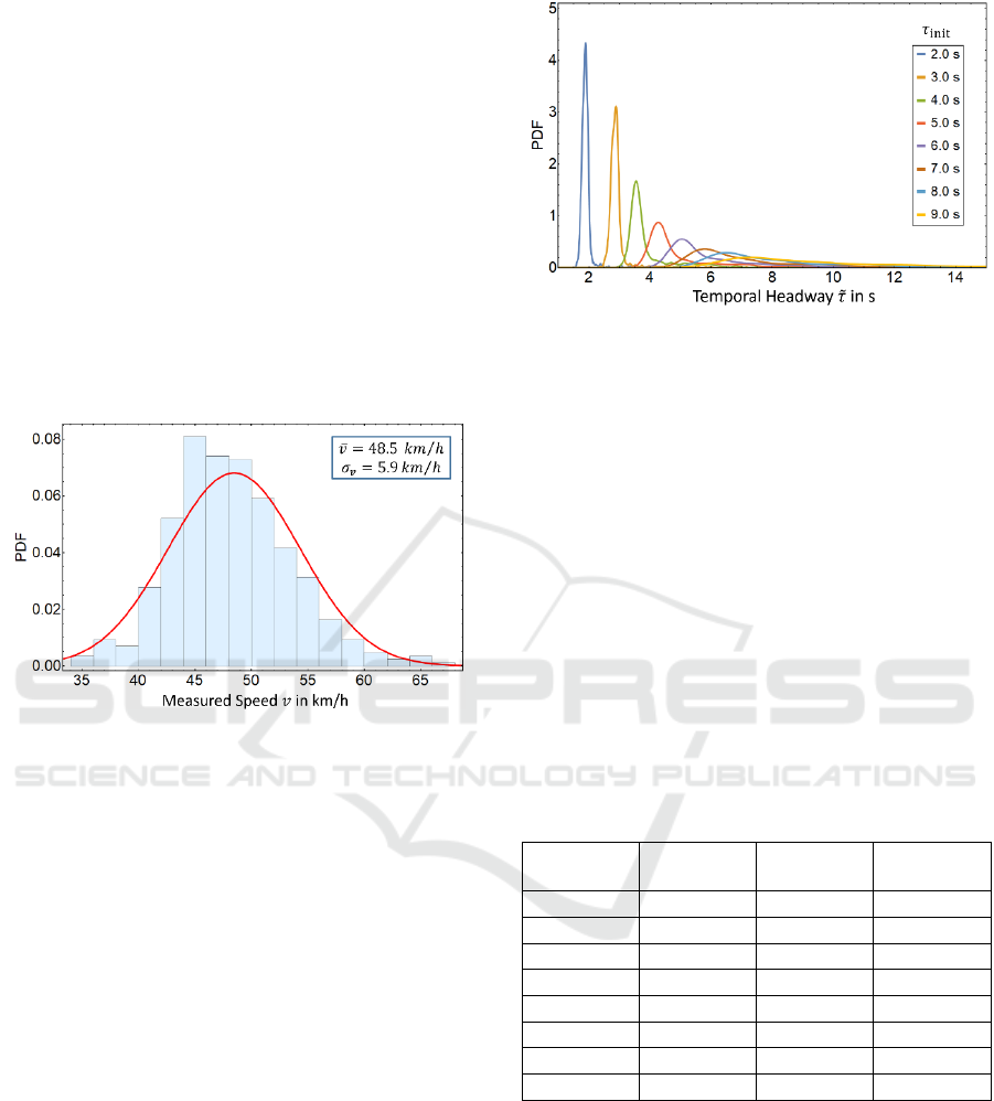
During the evaluation, only vehicle speeds in
flowing traffic were taken into account. The related
empirical speed histogram is shown in figure 3 (light
blue boxes). The single vehicle speeds are distributed
widely, which stays in contrast to the former
assumption
= const. It seems like the histogram
has an asymmetric shape. Due to the relatively small
dataset of 432 vehicles, this could also have been a
coincidence. That is why we chose a normal
distribution to fit the underlying data. With regard to
a simple solution on the one hand and taking into
account the basic characteristics of the dataset on the
other hand, the distribution adapts satisfactorily.
Figure 3: Empirical speed histogram of 432 vehicles in free
flow on an urban road in Duisburg, Germany. There is a
speed limit of 50 km/h. A normal distribution (red line)
satisfactorily fits the data. The underlying parameters for
mean and standard deviation
are shown in the upper
right corner. The error (±2 km/h) of the measured speed
dataset is of the same size as the histogram’s bin width.
2.3 Normal Distributed Free Flow
Parameter
Motivated through the empirical speed histogram in
figure 3, we randomised the value of the free flow
parameter
. It is now following a normal
distribution.
As a result, every car is initialised with its own
individual free flow speed. Of course, fluctuations are
still possible through the underlying stochastic
model. Mapping the empirical distribution from
subsection 2.2 to a speed limit of 30 km/h, delivers a
mean of approx. 29 km/h. However, the standard
deviation is expected to remain the same (~6 km/h).
Subsequently, the same procedure as in
subsection 2.1 takes place following the rules of the
Kerner-Klenov model.
Figure 4: Probability density function (PDF) against the
temporal headway at the intersection point
for
different initial temporal headways
. For each vehicle,
the free flow parameter
is not constant, but is
randomised following a normal distribution. All vehicles
are initialised at
(see figure 1). Due to this empirically
motivated modification, more softened distributions are
resulting, i.e. the statistical temporal headway scatters
within a wider range.
However, for this case, we obtain fundamentally
different distributions (figure 4) in comparison to the
previous case (figure 2). Now, they are much more
softened and the peak-like behavior is gone, i.e. the
statistical temporal headway scatters within a wider
range. With regard to a more quantitative explanation
mean, variance and skewness of the distributions are
listed in Table 2.
Table 2: Mean, variance and skewness of the distributions
shown in figure 4.
[s]
Mean
[s]
Variance
[s²]
Skewness
[s³]
2.0
1.91
0.07
7.26
3.0
2.96
0.29
5.28
4.0
4.04
1.31
3.20
5.0
5.17
2.87
2.54
6.0
6.18
3.64
2.45
7.0
7.28
5.23
2.35
8.0
8.18
5.27
1.33
9.0
9.45
7.88
1.09
3 DISCUSSION
Although the Kerner-Klenov model exhibits
stochastic components, the fluctuations for a
moderate traffic flow are very slight, obviously. Only
when the model is applied to bottleneck situations, the
characteristics of real traffic are reproduced
realistically and the fluctuations of the model
An Agent-based Approach to a Temporal Headway Development Statistics in Urban Traffic using Three-phase Theory
241
increase. Due to the slight model fluctuations, sharp
peaks are resulting (figure 2), i.e. the temporal
headway is not changing significantly within the
range from
to
. This behaviour does not seem
to be realistic at all. In Table 1 mean, variance and
skewness are listed to enable a quantitative point of
view.
Compared to other works, where often only
averaged empirical data over many cars is shown, our
dataset consists of single vehicle information. The
measurement took place on a bright day without any
precipitation in April 2018 on a straight road in
Duisburg, Germany exhibiting a speed limit of 50
km/h. Only vehicle speeds in flowing traffic were
taken into account. In order to make sure that the
driving behaviour of individual cars was not affected
by the measurement, the cameras were placed hidden.
Two road markings with a distance of 20 meters in
between served as an aid to determine speeds of
passing vehicles. Due to the associated averaging
process of the vehicle speeds within a range of 20
meters, an error of ±2 km/h should be taken into
account. This corresponds to the bin width of the
histogram shown in figure 3.
In order to obtain a more realistic behaviour
within the framework of a microscopic simulation, a
randomised free flow parameter
was chosen for
different initial temporal headways
(figure 4).
When comparing the different distributions of , it is
noticeable that they are getting wider (increasing
variance) with increasing
(table 2). However, the
skewness is continuously decreasing. This is due to
the safe space gap
of the Kerner-Klenov model,
which represents the lower limit of the gap between
two consecutive vehicles. If the gap is already small,
there are many more possibilities for an increase. The
bigger it becomes, the more balanced options there
are for the underlying agent leading to a more
symmetric shape of the related distribution. The mean
value of the temporal headway stays very close to
the initial value
.
It is interesting to see, that the results of
subsection 2.1 and subsection 2.3 differ not only in
variance, but also in their skewness (compare table 1
to table 2). Whereas a negative skewness is obtained
for a constant
, the skewness becomes positive
for a free flow parameter following a normal
distribution. A comparision of the mean values
shows, that both are systematically smaller than the
underlying initial value
.
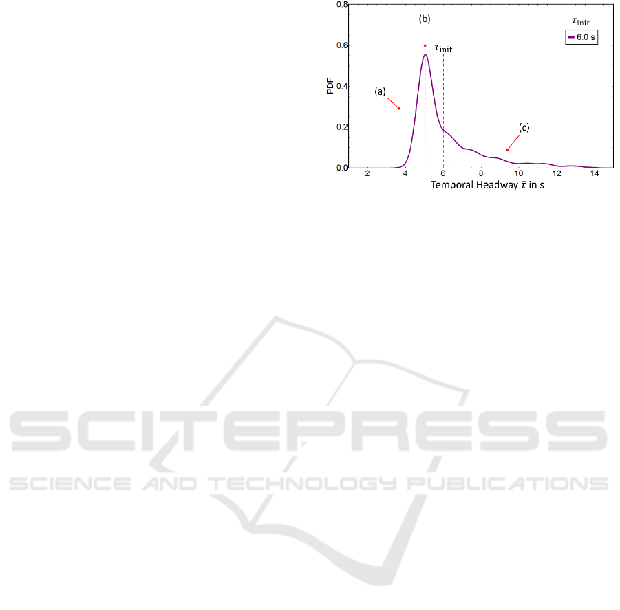
For the following qualitative discussion, we now
turn to figure 5 showing a single distribution of from
figure 4 (
= 6 s). It seems that the mode of the
Figure 5: Qualitative discussion on the PDF for
following a normal distribution. As an example, the
distribution for the simulation of
= 6 s has been chosen
(see figure 4), which is representative of all. Compared to
the PDF’s heavy tail towards larger temp. headways (c),
the distribution has a steep slope towards shorter (a). The
mode (b, black dashed line) is systematically smaller than
the underlying initial temp. headway
(red dashed line).
distribution is systematically smaller than the
underlying initial temporal headway
, i.e. most of
the cars within the analysed ensemble tend to close
the gap to their preceding vehicle. The distribution
has got a steep slope on its left-hand side. It looks as
if there is a lower limit relating to short temporal
headways for a given
, whereas the heavy tail’s
range towards larger temporal headways cannot be
determined clearly.
4 CONCLUSIONS
We found out that the typical probability density
function (PDF) describing the temporal headway
development do not have a symmetrical shape. A
heavy tail behaviour towards larger temporal
headways occurs, if the free flow parameter
of
the underlying Kerner-Klenov model follows a
normal distribution. This shape seems to be
qualitatively independent of the initial temporal
headway
. Providing this information to an
automated vehicle helps to find the most efficient
driving strategy for merging into the ongoing traffic.
We would like to compare our results to real
traffic temporal headway distributions. With regard to
the described scenario, we are developing a stationary
infrared sensor system including multiple units to
detect a large number of passing vehicles. Using the
generated data helps us to adjust the model’s
underlying functions and parameters in order to
describe real traffic more reliable. Furthermore, this
research is going to be shared within the “MEC-
ICAART 2019 - 11th International Conference on Agents and Artificial Intelligence
242

View“-project. The aim is to optimise the algorithm
finding the most efficient driving strategy for the
involved automated vehicle approaching the project’s
T-intersection.
ACKNOWLEDGEMENTS
The authors thank the partners for their support within
the project "MEC-View – Mobile Edge Computing
basierte Objekterkennung für hoch- und
vollautomatisiertes Fahren", funded by the German
Federal Ministry of Economics and Energy by
resolution of the German Federal Parliament.
REFERENCES
Chandler, R. E., Herman, R., Montroll, E. W., 1958. Traffic
dynamics: studies in car following. Operations
research, 6(2), 165-184.
Chmura, T., Herz, B., Knorr, F., Pitz, T., Schreckenberg,
M., 2014. A simple stochastic cellular automaton for
synchronized traffic flow, Physica A: Statistical
Mechanics and its Applications, 405, 332-337.
Hafstein, S. U. F., Chrobok, R., Pottmeier, A.,
Schreckenberg, M., C. Mazur, F., 2004. A high‐
resolution cellular automata traffic simulation model
with application in a freeway traffic information
system, Computer‐Aided Civil and Infrastructure
Engineering, 19(5), 338-350.
Kerner, B., 2000. Theory of breakdown phenomenon at
highway bottlenecks, Transportation Research Record:
Journal of the Transportation Research Board, (1710),
136-144.
Kerner, B. S., 2004. The Physics of Traffic, Springer.
Berlin, Heidelberg, New York.
Kerner, B. S., Klenov, S. L., 2009. Phase transitions in
traffic flow on multilane roads, Physical Review E,
80(5), 056101.
Kerner, B. S., 2013. The physics of green-wave breakdown
in a city, EPL, 102(2), 28010.
Kerner, B. S., 2017. Breakdown in Traffic Networks,
Springer. Berlin.
Krauss, S., Wagner, P., Gawron C., 1997. Metastable states
in a microscopic model of traffic flow. Physical Review
E, 55(5), 5597.
Nagel, K., Schreckenberg, M., 1992. A cellular automaton
model for freeway traffic. Journal de physique I, 2(12),
2221-2229.
Rickert, M., Nagel, K., Schreckenberg, M., Latour, A,
1996. Two lane traffic simulations using cellular
automata, Physica A: Statistical Mechanics and its
Applications, 231(4), 534-550
An Agent-based Approach to a Temporal Headway Development Statistics in Urban Traffic using Three-phase Theory
243
