Measuring the Data Efﬁciency of Deep Learning Methods

Hlynur Davíð Hlynsson, Alberto N. Escalante-B. and Laurenz Wiskott

Ruhr University Bochum, Universitätsstraße 150, 44801 Bochum, Germany

Keywords:

Data Efﬁciency, Deep Learning, Neural Networks, Slow Feature Analysis, Transfer Learning.

Abstract:

In this paper, we propose a new experimental protocol and use it to benchmark the data efﬁciency — perfor-

mance as a function of training set size — of two deep learning algorithms, convolutional neural networks

(CNNs) and hierarchical information-preserving graph-based slow feature analysis (HiGSFA), for tasks in

classiﬁcation and transfer learning scenarios. The algorithms are trained on different-sized subsets of the

MNIST and Omniglot data sets. HiGSFA outperforms standard CNN networks when the models are trained

on 50 and 200 samples per class for MNIST classiﬁcation. In other cases, the CNNs perform better. The re-

sults suggest that there are cases where greedy, locally optimal bottom-up learning is equally or more powerful

than global gradient-based learning.

1 INTRODUCTION

In recent years, we have seen convolutional neural

networks (CNN) dominate benchmark after bench-

mark for computer vision since the 2012 ImageNet

competition breakthrough (Krizhevsky et al., 2012).

These methods prosper with an abundance of labeled

data, and an abundance of data is often required for

acceptable results (Oquab et al., 2014). In contrast,

for most people, it is only necessary to see one pic-

ture of an Atlantic Pufﬁn to be able to identify cor-

rectly such a bird as one.

To be fair, we have a lot of prior experience. It is

easy to make a mental note: “a pufﬁn is a small black

and white bird with orange feet and a colorful beak”

because we have learned a useful representation of the

salient aspects of the image. Instead of being bogged

down by the details of every exact pixel value, as an

untrained AI might, we can focus our attention on the

most useful features of the image.

For this reason, investigations on the efﬁcacy of

methods to learn a concept from few samples are of-

ten done through the lens of representation learning

(Bengio et al., 2013), for example via transfer learn-

ing (Pan and Yang, 2010) or low-shot learning (Wang

et al., 2018).

In this work we consider a method to measure

data efﬁciency, the performance of an algorithm

as a function of the number of data points avail-

able during training time, which is an important as-

pect of machine learning (Kamthe and Deisenroth,

2017), (Al-Jarrah et al., 2015). We quantitatively

examine the performance of CNNs and hierarchi-

cal information-preserving graph-based slow feature

analysis (HiGSFA) (Escalante-B and Wiskott, 2016)

networks for varying training set sizes and for vary-

ing task types.

HiGSFA has been chosen because it is the most

recent supervised extensions of slow feature analy-

sis (SFA) and has shown promise in visual processing

with a notable distinction from CNNs: the computa-

tion layers are trained in a "greedy" layer-wise man-

ner instead of via gradient descent (Escalante-B and

Wiskott, 2016).

The methods are applied to visual tasks: a simple

version of the MNIST classiﬁcation task, where we

vary the number of training points, and increasingly

difﬁcult tasks constructed from the Omniglot dataset.

Our contribution in this work is a novel experimen-

tal protocol for evaluation of transfer learning applied

to experimentally evaluate CNNs with the slowness-

based HiGSFA.

2 RELATED WORK

Gathering data can be quite costly, so the question

"how much is enough" has been considered in lit-

erature ranging from classical statistics (Krishnaiah,

1980) over pattern recognition (Raudys and Jain,

1991) to experimental design (Beleites et al., 2013).

As data plays a central role in machine learning as

well, the study of its effective use has garnered atten-

tion from all branches of the ﬁeld.

In a similar vein as our work, (Lawrence et al.,

1998) analyze the effect of generalization when the

Hlynsson, H., Escalante-B., A. and Wiskott, L.

Measuring the Data Efﬁciency of Deep Learning Methods.

DOI: 10.5220/0007456306910698

In Proceedings of the 8th International Conference on Pattern Recognition Applications and Methods (ICPRAM 2019), pages 691-698

ISBN: 978-989-758-351-3

691

number of sample points are varied for supervised

learning tasks. Equipped with the prior that super-

vised learning methods’ performance obeys the in-

verse power law, (Figueroa et al., 2012) trained a

model to predict the classiﬁcation accuracy of a model

given a number of inputs.

Transfer learning straddles the intersection be-

tween supervised learning and unsupervised learning,

where the focus is uncovering representations that are

both general and also useful for particular applica-

tions. The Omniglot data set we consider was in-

troduced in (Lake et al., 2015) and has been popular

for developing transfer learning methods (Bertinetto

et al., 2016), (Edwards and Storkey, 2016), (Schwarz

et al., 2018).

With its sparse rewards and problems of credit as-

signment, reinforcement learning (RL) has a partic-

ular need for data efﬁciency, motivating such early

works as prioritized sweeping (Moore and Atkeson,

1993). More recently, (Riedmiller, 2005) designed

the neural-ﬁtted Q-learner for data efﬁciency. This

method has been successfully combined with deep

auto-encoder representations for visual RL (Lange

and Riedmiller, 2010). Deep Q-Networks have made

better still use of data for RL by combining expe-

rience replay, target networks, reward clipping and

frame skipping (Mnih et al., 2013) (Mnih et al., 2015).

SFA was introduced in 2002 by Wiskott and Se-

jnowski as an unsupervised learning method of tem-

porally invariant features (Wiskott and Sejnowski,

2002). These features can be learned hierarchically in

a bottom-up manner, reminiscent of deep CNNs: slow

features are learned on spatial patches of the input and

then passed to another layer for slow feature learning.

The method is then called hierarchical slow feature

analysis (HSFA) and has attracted attention in neuro-

science for plausible modeling of grid, place, spatial-

view, and head-direction cells (Franzius et al., 2007).

For labeled data, the method admits a supervised

extension in the form of graph-based SFA (GSFA)

(Escalante and Wiskott, 2013). Information is often

lost in early layers of hierarchical SFA — that could

contribute to a globally slower signal — prompt-

ing the development of HiGSFA (Escalante-B and

Wiskott, 2016).

Deep learning extensions of SFA is currently an

active research area. The SFA problem is solved

with stochastic optimization in Power-SFA (Schüler

et al., 2018). A differentiable whitening layer is con-

structed, allowing for a non-linear expansion of the

input to be learned with backpropagation. Another

recent method, SPIN (Pfau et al., 2018) learns eigen-

functions of linear operators with deep learning meth-

ods and can be applied to the SFA problem as well.

3 METHODS

Below we describe the novel experimental setup as

well as the methods being evaluated using the setup.

For the remainder of the article we assume CNNs to

be well-known and understood but we can recom-

mend (CS231n, 2017) as a good pedagogical intro-

duction to the method.

3.1 HiGSFA

HiGSFA belongs to a class of methods motivated by

the slowness principle, which is based on the assump-

tion that important aspects vary more slowly than

unimportant ones (Sun et al., 2014). This model takes

as input data points such that data point x

is node n in

an undirected graph with weight v(n). This can con-

trol the relative weight each data point has during the

training but we set it as uniformly 1 is our experiments

below.

The edge between nodes n and n

is γ

n,n

and sig-

niﬁes a relationship between the data. This could be

their spatial or temporal proximities or whether they

belong to the same class.

For instance, during our classiﬁcation tasks below,

we set:

n,n

(

1, if n and n

in same class

0, otherwise

(1)

Given a function space F with elements g

, we

learn slowly varying features y

(n) = g

) of the

data by solving the optimization problem (Escalante

and Wiskott, 2013):

minimize

n,n

∑

n,n



(n) − y

)



subject to

∑

(n) = 0

∑

(n))

= 1

∑

(n)y

(n) = 0, j

< j

where Q =

∑

, R =

∑

n,n

(2)

The ﬁrst constraint secures weighted zero mean,

the second constraint secures weighted unit variance

and the third one secures weighted decorrelation and

order.

To reduce computational complexity, we extract

features of the data hierarchically. Similarly to CNNs,

we extract features from F × F patches of the image

ICPRAM 2019 - 8th International Conference on Pattern Recognition Applications and Methods

692

data in the ﬁrst layer, then extract features of F

× F

patches of the output features in the next layer and so

on. The layers are trained by solving the optimization

problem, one layer at a time, from the input layer to

the output layer. The layer-wise parameters can be

shared.

As we can experience information-loss while do-

ing these layer-wise optimizations, an information-

preserving mechanism is added. The cost function is

minimized locally, so we can experience information-

loss if dimensions are discarded that do not minimize

the function on a local level — but could conceivably

be better for the overall problem.

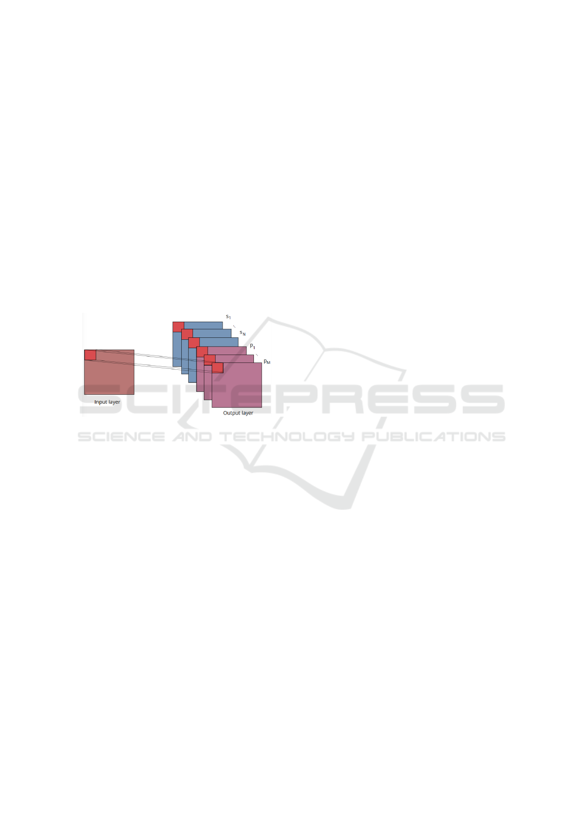
For each layer (ﬁgure 1), a threshold is placed on

the features with respect to their slowness. If an out-

put feature or features would be too fast, we replace

them by the most variance-preserving PCA features.

Each layer thus outputs a combination of slow fea-

tures and PCA features.

Figure 1: HiGSFA network layer. The feature generation is

similar to that of the CNN. The layer outputs N channels of

slow features and M channels of PCA features. The num-

ber of PCA channels features is either ﬁxed beforehand or

determined by replacing a number M of the SFA features

whose slowness (cost function in eq. 2) exceeds a given

threshold.

3.2 General Description of Protocol

The performance of two hypothesis h

and h

, not

necessarily from the same hypothesis set H , is

compared on a classiﬁcation task. The learning

curves of the two hypothesis are plotted as a function

of the number of data points in the training set. This

can be done simply by taking an increasing number

of training points per class as we evaluate using

MNIST, below.

Alternatively, the number of training points per

class are kept constant and the number of classes

are varied. The relationship training and test set

distributions is also altered, such that the task ranges

from classical classiﬁcation to transfer learning. We

report a comparison of methods below using this

scheme on the Omniglot data set.

3.3 Evaluation on MNIST

First, we compare classiﬁcation accuracies on

MNIST (LeCun et al., 1998) as a function of the num-

ber of samples per class used during training. The im-

ages have a dimension of 28 × 28 pixels. For 100 it-

erations, we choose random samples from each class

and use a thousand unused samples from each class

for validation. Finally, the models are tested on the

classic 10 thousand test images.

3.3.1 Architectures

We constructed a two-layer HiGSFA network with

circa 13k parameters (the number is stochastic and

changes from training set to training set), extracting

400 features from the data. The ﬁrst layer has a ﬁlter

size of 5 × 5 and a stride of 2, extracting 25 features

for each spatial patch. The second layer has a ﬁlter

size of 4 × 4 and a stride of 2, extracting 16 features

for each spatial patch.

The output of the ﬁrst layer is concatenated with a

copy of itself, where each element x is replaced with

|x|

0.8

, doubling the number of channels and giving us

nonlinearity. If the value of the objective function is

larger than a threshold of 1.99, we select PCA fea-

tures. This upper bound is motivated by the fact that

non-predictive, white noise features take a value of

2 in the objective function (Creutzig and Sprekeler,

2008). The parameters within each layer are shared.

A single-layer softmax neural network was trained on

the features of the second layer to handle classiﬁca-

tion, which has 4010 parameters.

Two standard CNNs were constructed as well, one

with the constraint to have a similar number of param-

eters as the HiGSFA network, and another with an

amount closer to what is seen in practice on similar

datasets. That is to say, the smaller CNN corresponds

to the HiGSFA network.

We call the smaller network CNN-1 which has

10,032 trainable parameters, excluding the number in

the ﬁnal layer for classiﬁcation. The tasks have vary-

ing numbers of classes to be predicted, causing the

classiﬁcation layer to have varying numbers of param-

eters. CNN-1 has three convolutional layers, each one

followed by ReLU and max pooling, the ﬁrst two with

8 channels and the last one with 16. They are followed

by a fully connected classiﬁcation layer, using a soft-

max activation function. The ﬁrst convolutional layer

has a ﬁlter size of 7×7, and the other two have a ﬁlter

size of 5 × 5. The convolutional layers have a stride

of 1 and the max pooling layers have a stride of 2.

We call the larger network CNN-2, with 116,214

parameters (not counting the classiﬁcation layer). It

is the same as CNN-1 except the convolutional layers

Measuring the Data Efﬁciency of Deep Learning Methods

693

have twice the number of channels, and a dense layer

with 150 units is added before the classiﬁcation layer.

Note that the parameter conﬁgurations of both

HiGSFA and CNNs have not been optimized for the

best performance on the tasks below. They were de-

signed to be lightweight according to general best

practices (Hadji and Wildes, 2018) (Escalante-B and

Wiskott, 2016). This allows for more trials and tighter

conﬁdence bounds while achieving fair performance

on the tasks.

3.4 Evaluation on Omniglot

Omniglot is a handwritten character dataset consist-

ing of 50 alphabets with 14 to 55 characters each, each

character having 20 samples (Lake et al., 2015). The

alphabets vary from real alphabets, such as Greek, to

ﬁctional ones, such as Alienese (from the TV show

“Futurama”). Each sample was drawn by a differ-

ent person for this dataset. It is typically split into 30

training alphabets, and 20 testing alphabets. Note that

the training-testing split separates the alphabets; all

samples originating from all characters from a given

alphabet appear in either the training set or the test set

but not both. This makes it a transfer learning task

as the training and test data set samples drawn from

separate distributions.

In the original work using the dataset, the meth-

ods were ﬁrst trained on the 30 background alpha-

bets, and then a 20 way one shot classiﬁcation task

was performed. Two samples are taken from each of

20 characters from random evaluation alphabets. One

sample is placed in what we’ll call a probe set, and

the other in a target set. The methods then try to ﬁnd

the corresponding sample in the target set that is the

same character as any given sample in the probe set.

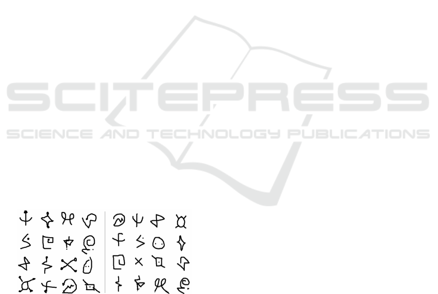
Figure 2: 16 way one shot classiﬁcation. Symbols on the

left are presented to the algorithm, one at a time, and the

task is to ﬁnd the same character from the symbols on the

right.

In the vein of the original Omniglot task, we com-

pare several models in three challenges. In all chal-

lenges, we do 16 way one shot classiﬁcation using

1-nearest-neighbor (1-NN) under the Euclidean dis-

tance. The challenges differ in how the test set is re-

lated to the training set:

3.4.1 Challenge 0

From 16 random characters used for training, we take

two samples that the models were trained on. These

samples are placed in two sets, the probe and target

sets, such that each set contains one sample of each

character. The model under consideration extracts

features from each image. We then iterate through

each feature vector from images in the probe set and

ﬁnd the closest feature vector from the target set. If

those two vectors belong to images of the same class,

then we count it as a success.

3.4.2 Challenge 1

Same as above, but we take characters used during

training for the probe set and perform classiﬁcation

on samples that were not used during the training.

3.4.3 Challenge 2

Same again, but now we do the classiﬁcation on char-

acters that do not belong to alphabets used during

training.

3.4.4 Omniglot Architectures

All model architectures are the same for MNIST

and Omniglot, but the Omniglot images are resized

to 35 × 35, having the effect that HiGSFA outputs

784 features. The number of model parameters does

not change as the weights are shared for the image

patches. The HiGSFA features used for classiﬁcation

are simply the 784 output features and we do not train

a neural network classiﬁer on them.

The total number of parameters in the CNNs de-

pend on the number of training classes, due to the

classiﬁcation layer. We ﬁx the number of alphabets to

8 and vary the number of characters per class to be 4,

6, 8, 10, 12 and vice versa. The number of parameters

for CNN-1 range between 18k and 35k, and for CNN-

2 range between 121k and 130. If we do not count the

parameters from the ﬁnal classiﬁcation layer, then the

number of parameters for CNN-1 for these tasks is

always 10,032 and the number for CNN-2 is 116,214.

After training the CNNs, we perform feature ex-

traction by intercepting the output of the second-to-

last layer. Here the assumption is that CNNs learn

a representation for the classiﬁcation layer (Razavian

et al., 2014). We are then interested in comparing the

strength of HiGSFA and CNN representations when

used by a 1-NN classiﬁer.

ICPRAM 2019 - 8th International Conference on Pattern Recognition Applications and Methods

694

Table 1: MNIST Accuracies. The percentage of correctly classiﬁed samples on the test set along with the standard error of

the mean (SEM).

Samples HiGSFA CNN-1 CNN-2

Acc. Std. Acc. Std. Acc. Std.

5 35.683 ± 0.430 72.361 ± 0.365 72.320 ± 0.094

10 75.736 ± 0.222 80.392 ± 0.241 79.551 ± 0.175

50 92.970 ± 0.050 90.320 ± 0.101 91.465 ± 0.070

200 96.246 ± 0.027 94.672 ± 0.062 95.648 ± 0.051

500 97.188 ± 0.013 96.579 ± 0.046 97.308 ± 0.054

2000 97.887 ± 0.009 98.247 ± 0.020 98.571 ± 0.023

6000 98.134 ± 0.008 98.687 ± 0.014 98.949 ± 0.015

3.4.5 Training

The models were trained on varying amounts of sam-

ples per character. The HiGSFA network was trained

to solve the optimization problem on each image

patch, one layer at a time. All neural networks were

trained in Keras (Chollet et al., 2015) using ADAM

(Kingma and Ba, 2014), with default parameters, to

minimize cross-entropy.

After each epoch, the error was calculated on the

validation set. Early stopping was performed after

the validation error had increased four times in to-

tal during the training. The training for Omniglot is

the same, except instead of early stopping, the CNNs

were trained for 20 epochs in all cases.

4 RESULTS

4.1 MNIST Results

We trained the models using 5, 10, 50, 200, 2000 or

4000 samples per digit. In table 1, we see the statistics

from 100 runs, where the models were trained from

random initializations, evaluated and tested. The con-

volutional networks have the highest accuracies when

there are 2000 or more samples per class and when

there are only 5 or 10 samples per class.

However, HiGSFA has a higher accuracy than the

CNN with a similar number of parameters for 500

samples per class. Furthermore, HiGSFA has higher

accuracies than both CNNs for 200 and 50 samples

per class. The CNN with a larger number of parame-

ters always has higher prediction accuracies than the

one with a lower number of parameters.

4.2 Omniglot Results

The 1-NN classiﬁer uses the second-to-last CNN

outputs or HiGSFA features. We ﬁx either the

number of alphabets, or characters-per-alphabet,

to be 8 and vary the other number from 4 to

12 in increments of 2. The number of sam-

ples per character is either 4 or 16. The largest

total number (alphabets × characters per alphabet ×

samples per character) of samples used for training is

1536 and the lowest is 128.

In ﬁgure 3, we see the average of all the runs

over the different samples per characters and number

of classes. In all of the challenges, the CNNs have

higher accuracies than HiGSFA. On average, CNN-2

has higher accuracies in challenges 0 and 2. Neither

CNN achieves signiﬁcantly better accuracy than the

other in challenge 1.

5 DISCUSSION AND

CONCLUSION

The work of this paper is intended to facilitate under-

standing of algorithms from the point of view of hav-

ing particularly low numbers of samples. We present

simple-to-implement challenges that allow for evalua-

tion of data efﬁciency in the context of representation

learning.

For the models experimented on, we see that

the CNNs usually perform better, but HiGSFA out-

performs the CNNs on 50 and 200 sample training

sets from the MNIST data. One can speculate that

the default CNN architectures ensure generalization

through max-pooling whereas SFA mostly learns to

generalize from a moderately sized data set.

Another explanation for the different ranges of

comparative performance optima is the choice of

delta-threshold of HiGSFA. The method overesti-

mates the slowness of the slowest features when it has

too few samples. This has the effect that fewer PCA

features are selected for a lower number of samples.

On the other hand, with more than 200 samples, there

could be too many PCA features chosen. Setting the

number of slow features to be a constant for all sam-

Measuring the Data Efﬁciency of Deep Learning Methods

695

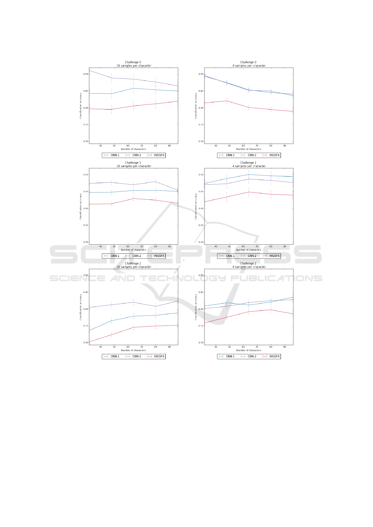
Figure 3: Classiﬁcation Accuracies. There are either 8 alphabets and we vary the characters per alphabet, or vice versa. The

error bars indicate the standard error of the mean. These plots are best viewed in color.

ple sizes could be better for robustness than ﬁxing the

delta threshold.

Notice the trend in challenge 0: the accuracy goes

down as the number of samples increases. This is due

to the samples used for the probe and target sets being

drawn from the training set and we are training and

testing on larger sets as we move from left to right.

Overall, for the Omniglot challenges, the accura-

cies of the CNNs lie comfortably above the HiGSFA

accuracies, but it’s not always discernible whether the

larger or the smaller CNN performs better. An ex-

planation for this could be that the tasks are not difﬁ-

cult enough for more parameters to be necessary. The

local optimality of GSFA could result in an insufﬁ-

ciently robust or transferable representation if there

are many classes and few samples per class.

These challenges are more complicated set of

classiﬁcation tasks than the MNIST ones, with a

ICPRAM 2019 - 8th International Conference on Pattern Recognition Applications and Methods

696

larger number of classes overall. This give CNNs an

opportunity to take advantage of having been trained

directly for classiﬁcation when they are presented a

similar task. Although HiGSFA takes advantage of

class labels, it suffers in comparison for not taking

into account the downstream task during training.

For future work, a complete extension of the ex-

periments here could include an analysis on the effect

that different type of data would have on the perfor-

mance. This would yield further insight than vary-

ing the number of rather homogeneous data used for

training. Additionally, the performance of a wider ar-

ray of popular methods can be compared.

More types of benchmarks for comparing differ-

ent models over varying training set sizes would be

helpful for this kind of research. Knowledge gained

from them would as well allow practitioners to choose

the right model for the scale and type of the problem

they wish to solve. These experiments give rise to the

question: how can these methods with their different

strengths and weaknesses proﬁt from each other?

REFERENCES

Al-Jarrah, O. Y., Yoo, P. D., Muhaidat, S., Karagiannidis,

G. K., and Taha, K. (2015). Efﬁcient machine learning

for big data: A review. Big Data Research, 2(3):87–

93.

Beleites, C., Neugebauer, U., Bocklitz, T., Krafft, C., and

Popp, J. (2013). Sample size planning for classiﬁca-

tion models. Analytica chimica acta, 760:25–33.

Bengio, Y., Courville, A., and Vincent, P. (2013). Represen-

tation learning: A review and new perspectives. IEEE

transactions on pattern analysis and machine intelli-

gence, 35(8):1798–1828.

Bertinetto, L., Henriques, J. F., Valmadre, J., Torr, P., and

Vedaldi, A. (2016). Learning feed-forward one-shot

learners. In Advances in Neural Information Process-

ing Systems, pages 523–531.

Chollet, F. et al. (2015). Keras. https://keras.io.

Creutzig, F. and Sprekeler, H. (2008). Predictive coding

and the slowness principle: An information-theoretic

approach. Neural Computation, 20(4):1026–1041.

CS231n, S. (2017). Convolutional neural networks for vi-

sual recognition.

Edwards, H. and Storkey, A. (2016). Towards a neural

statistician. arXiv preprint arXiv:1606.02185.

Escalante, A. N. and Wiskott, L. (2013). How to

solve classiﬁcation and regression problems on high-

dimensional data with a supervised extension of slow

feature analysis. Journal of Machine Learning Re-

search, 14(1):3683–3719.

Escalante-B, A. N. and Wiskott, L. (2016). Improved

graph-based SFA: Information preservation comple-

ments the slowness principle. CoRR.

Figueroa, R. L., Zeng-Treitler, Q., Kandula, S., and Ngo,

L. H. (2012). Predicting sample size required for clas-

siﬁcation performance. BMC medical informatics and

decision making, 12(1):8.

Franzius, M., Sprekeler, H., and Wiskott, L. (2007). Slow-

ness and sparseness lead to place, head-direction,

and spatial-view cells. PLoS computational biology,

3(8):e166.

Hadji, I. and Wildes, R. P. (2018). What do we under-

stand about convolutional networks? arXiv preprint

arXiv:1803.08834.

Kamthe, S. and Deisenroth, M. P. (2017). Data-efﬁcient

reinforcement learning with probabilistic model pre-

dictive control. arXiv preprint arXiv:1706.06491.

Kingma, D. P. and Ba, J. (2014). Adam: A

method for stochastic optimization. arXiv preprint

arXiv:1412.6980.

Krishnaiah, P. R. (1980). Handbook of statistics, volume 31.

Motilal Banarsidass Publishe.

Krizhevsky, A., Sutskever, I., and Hinton, G. E. (2012). Im-

agenet classiﬁcation with deep convolutional neural

networks. In Advances in neural information process-

ing systems, pages 1097–1105.

Lake, B. M., Salakhutdinov, R., and Tenenbaum, J. B.

(2015). Human-level concept learning through proba-

bilistic program induction. Science, 350(6266):1332–

1338.

Lange, S. and Riedmiller, M. (2010). Deep auto-encoder

neural networks in reinforcement learning. In The

2010 International Joint Conference on Neural Net-

works (IJCNN), pages 1–8. IEEE.

Lawrence, S., Giles, C. L., and Tsoi, A. C. (1998). What

size neural network gives optimal generalization?

convergence properties of backpropagation. Techni-

cal report.

LeCun, Y., Bottou, L., Bengio, Y., and Haffner, P. (1998).

Gradient-based learning applied to document recogni-

tion. Proceedings of the IEEE, 86(11):2278–2324.

Mnih, V., Kavukcuoglu, K., Silver, D., Graves, A.,

Antonoglou, I., Wierstra, D., and Riedmiller, M.

(2013). Playing atari with deep reinforcement learn-

ing. arXiv preprint arXiv:1312.5602.

Mnih, V., Kavukcuoglu, K., Silver, D., Rusu, A. A., Veness,

J., Bellemare, M. G., Graves, A., Riedmiller, M., Fid-

jeland, A. K., Ostrovski, G., et al. (2015). Human-

level control through deep reinforcement learning.

Nature, 518(7540):529.

Moore, A. W. and Atkeson, C. G. (1993). Prioritized sweep-

ing: Reinforcement learning with less data and less

time. Machine learning, 13(1):103–130.

Oquab, M., Bottou, L., Laptev, I., and Sivic, J. (2014).

Learning and transferring mid-level image represen-

tations using convolutional neural networks. In Pro-

ceedings of the IEEE conference on computer vision

and pattern recognition, pages 1717–1724.

Pan, S. J. and Yang, Q. (2010). A survey on transfer learn-

ing. IEEE Transactions on knowledge and data engi-

neering, 22(10):1345–1359.

Pfau, D., Petersen, S., Agarwal, A., Barrett, D., and

Stachenfeld, K. (2018). Spectral inference networks:

Measuring the Data Efﬁciency of Deep Learning Methods

697

Unifying spectral methods with deep learning. CoRR,

abs/1806.02215.

Raudys, S. J. and Jain, A. K. (1991). Small sample size ef-

fects in statistical pattern recognition: Recommenda-

tions for practitioners. IEEE Transactions on Pattern

Analysis & Machine Intelligence, (3):252–264.

Razavian, A. S., Azizpour, H., Sullivan, J., and Carlsson,

S. (2014). CNN features off-the-shelf: an astounding

baseline for recognition. CoRR, abs/1403.6382.

Riedmiller, M. (2005). Neural ﬁtted q iteration–ﬁrst ex-

periences with a data efﬁcient neural reinforcement

learning method. In European Conference on Ma-

chine Learning, pages 317–328. Springer.

Schüler, M., Hlynsson, H. D., and Wiskott, L. (2018).

Gradient-based training of slow feature analysis by

differentiable approximate whitening. arXiv preprint

arXiv:1808.08833.

Schwarz, J., Luketina, J., Czarnecki, W. M., Grabska-

Barwinska, A., Teh, Y. W., Pascanu, R., and Had-

sell, R. (2018). Progress & compress: A scalable

framework for continual learning. arXiv preprint

arXiv:1805.06370.

Sun, L., Jia, K., Chan, T.-H., Fang, Y., Wang, G., and Yan,

S. (2014). Dl-sfa: deeply-learned slow feature analy-

sis for action recognition. In Proceedings of the IEEE

conference on computer vision and pattern recogni-

tion, pages 2625–2632.

Wang, Y.-X., Girshick, R., Hebert, M., and Hariharan, B.

(2018). Low-shot learning from imaginary data. arXiv

preprint arXiv:1801.05401.

Wiskott, L. and Sejnowski, T. J. (2002). Slow feature anal-

ysis: Unsupervised learning of invariances. Neural

computation, 14(4):715–770.

ICPRAM 2019 - 8th International Conference on Pattern Recognition Applications and Methods

698