
Vertical and Horizontal Distances to Approximate Edit Distance
for Rooted Labeled Caterpillars
Kohei Muraka, Takuya Yoshino and Kouichi Hirata
Kyushu Institute of Technology, Kawazu 680-4, Iizuka 820-8502, Japan
Keywords:
Edit Distance, Rooted Labeled Caterpillar, Vertical Distance, Horizontal Distance, String Edit Distance,
Multiset Edit Distance.
Abstract:
A rooted labeled caterpillar (caterpillar, for short) is a rooted labeled tree transformed to a rooted path (called
a backbone) after removing all the leaves in it and we can compute the edit distance between caterpillars in
quartic time. In this paper, we introduce two vertical distances and two horizontal distances for caterpillars.
The former are based on a string edit distance between the string representations of the backbones and the
latter on a multiset edit distance between the multisets of labels occurring in all the leaves. Then, we show that
these distances give both lower bound and upper bound of the edit distance and we can compute the vertical
distances in quadratic time and the horizontal distances in linear time under the unit cost function.
1 INTRODUCTION
Comparing tree-structured data such as HTML and
XML data for web mining or RNA and glycan data for
bioinformatics is one of the important tasks for data
mining. The most famous distance measure between
rooted labeled unordered trees (trees, for short) is the
edit distance (Tai, 1979). The edit distance is formu-
lated as the minimum cost of edit operations, con-
sisting of a substitution, a deletion and an insertion,
applied to transform a tree to another tree. Unfor-
tunately, the problem of computing the edit distance
between trees is MAX SNP-hard (Zhang and Jiang,
1994), even if trees are binary or height 2 (Akutsu
et al., 2013; Hirata et al., 2011).
A caterpillar (cf. (Gallian, 2007)) is a tree trans-
formed to a rooted path after removing all the leaves
in it. Recently, Muraka et al. (Muraka et al., 2018)
have shown that we can compute the edit distance
between caterpillars in O(h
2
λ
2
) time, where h is the
maximum height and λ is the maximum number of
leaves in caterpillars. Hence, the problem is quartic-
time tractable with respect to the maximum number
of nodes, which is not efficient well.
As an efficient distance comparing caterpillars,
histogram distances such as a path histogram dis-
tance (Kawaguchi et al., 2018), a complete subtree
histogram distance (Akutsu et al., 2013; Yoshino
et al., 2018) and an LCA histogram distance (Yoshino
et al., 2018) have developed. Whereas these distances
are metrics for caterpillars and we can compute them
more efficiently (linear or quadratic time) than the edit
distance (quartic time), they are incomparable with
the edit distance in both theoretical and experimental.
In order to approximate the edit distance for cater-
pillars efficiently, in this paper, we introduce two ver-
tical distances d
V
and d
∗
V
based on a string edit dis-
tance and two horizontal distances d
H
and d
∗
H
based
on a multiset edit distance. Here, the multiset edit dis-
tance coincides with a famous bag distance (Deza and
Deza, 2016) if we adopt a unit cost function.
Let C
1
and C
2
be caterpillars. Then, d
V
(C
1
,C
2
) is
the string edit distance between the string representa-
tions of the backbones ofC
1
and C
2
, and d
∗
V
(C
1
,C
2
) is
the sum of d
V
(C
1
,C
2
), the multiset edit distance be-
tween the multisets on labels occurring in the leaves
of the endpoints of the backbones in C
1
and C
2
and
the costs of deleting the remained leaves in C
1
and
inserting the remained leaves in C
2
. Also d
H
(C
1
,C
2
)
is the multiset edit distance between the multisets of
labels occurring in all the leaves of C
1
and C
2
, and
d
∗
H
(C
1
,C
2
) is the sum of d
H
(C
1
,C
2
), the cost of the
correspondence between the roots of C
1
and C
2
and
the costs of deleting nodes in the backbone in C
1
and
inserting nodes in the backbone in C
2
.
Then, we show that these distances provide the
following lower bound and upper bound of the edit
distance τ
TAI
(C
1
,C
2
) between C
1
and C
2
.
max{d
V
(C
1
,C
2
),d
H
(C
1
,C
2
)}
≤ τ
TAI
(C
1
,C
2
) ≤ min{d
∗
V
(C
1
,C
2
),d
∗
H
(C
1
,C
2
)}.
590
Muraka, K., Yoshino, T. and Hirata, K.
Vertical and Horizontal Distances to Approximate Edit Distance for Rooted Labeled Caterpillars.
DOI: 10.5220/0007387205900597
In Proceedings of the 8th International Conference on Pattern Recognition Applications and Methods (ICPRAM 2019), pages 590-597
ISBN: 978-989-758-351-3
Copyright
c
2019 by SCITEPRESS – Science and Technology Publications, Lda. All rights reser ved

Furthermore, if we adopt the unit cost function, then
we can compute d
V
(C
1
,C
2
), d
∗
V
(C
1
,C
2
), d
H
(C
1
,C
2
)
and d
∗
H
(C
1
,C
2
) in O(h
2
) time, O(h
2
+ λ) time, O(λ)
time and O(λ + h) time, respectively. Hence, we can
compute the vertical distances in quadratic time and
the horizontal distances in linear time with respect to
the number of nodes.
Finally, we give experimental results to evaluate
the running time and the approximation for caterpil-
lars in real data.
2 PRELIMINARIES
A tree T is a connected graph (V,E) without cycles,
where V is the set of vertices and E is the set of edges.
We denote V and E by V(T) and E(T). The size of
T is |V| and denoted by |T|. We sometime denote
v ∈ V(T) by v ∈ T. We denote an empty tree (
/
0,
/
0) by
/
0. A rooted tree is a tree with one node r chosen as its
root. We denote the root of a rooted tree T by r(T).
Let T be a rooted tree such that r = r(T) and
u,v, w∈ T. We denote the unique path from r to v, that
is, the tree (V
′
,E
′
) such that V
′
= {v
1
,... , v
k
}, v
1
= r,
v
k
= v and (v
i
,v
i+1
) ∈ E
′
for every i (1 ≤ i ≤ k − 1),
by UP
r
(v).
The parent of v(6= r), which we denote by par(v),
is its adjacent node on UP
r
(v) and the ancestors of
v(6= r) are the nodes on UP
r
(v)−{v}. We say that u is
a child of v if v is the parent of u and u is a descendant
of v if v is an ancestor of u. We denote the set of
children of v by ch(v) and that v is a ancestor of u
by u ≤ v. We call a node with no children a leaf and
denote the set of all the leaves in T by lv(T).
A rooted path P is a rooted tree
({v
1
,... , v
n
},{(v
i
,v
i+1
) | 1 ≤ i ≤ n − 1}) such
that r(P) = v
1
. We call the node v
n
(the leaf of P) an
endpoint of P and denote it by e(P).
The degree of v, denoted by d(v), is the number of
children of v, and the degree of T, denoted by d(T), is
max{d(v) | v ∈ T}. The height of v, denoted by h(v),
is max{|UP
v
(w)| | w ∈ lv(T[v])}, and the height of T,
denoted by h(T), is max{h(v) | v ∈ T}.
We say that u is to the left of v in T if pre(u) ≤
pre(v) for the preorder number pre in T and post(u) ≤
post(v) for the postorder number post in T. We say
that a rooted tree is ordered if a left-to-right order
among siblings is given; unordered otherwise. We say
that a rooted tree is labeled if each node is assigned a
symbol from a fixed finite alphabet Σ. For a node v,
we denote the label of v by l(v), and sometimes iden-
tify v with l(v). In this paper, we call a rooted labeled
unordered tree a tree simply.
Definition 1 (Caterpillar (cf., (Gallian, 2007))). We
say that a tree is a caterpillar if it is transformed to a
rooted path after removing all the leaves in it. For a
caterpillarC, we call the remained rooted path a back-
bone of C and denote it by bb(C).
It is obvious that r(C) = r(bb(C)) and V(C) =
bb(C) ∪ lv(C) for a caterpillar C, that is, every node
in a caterpillar is either a leaf or an element of the
backbone.
Next, we introduce a tree edit distance and a Tai
mapping.
Definition 2 (Edit operations (Tai, 1979)). The edit
operations of a tree T are defined as follows, see Fig-
ure 1.
1. Substitution: Change the label of the node v in T.
2. Deletion: Delete a node v in T with parent v
′
,
making the children of v become the children of
v
′
. The children are inserted in the place of v as
a subset of the children of v
′
. In particular, if v is
the root in T, then the result applying the deletion
is a forest consisting of the children of the root.
3. Insertion: The complement of deletion. Insert a
node v as a child of v
′
in T making v the parent of
a subset of the children of v
′
.
Substitution (v 7→ w)
v
7→
w
Deletion (v 7→ ε)
v
′
v
7→
v
′
Insertion (ε 7→ v)
v
′
7→
v
′
v
Figure 1: Edit operations for trees.
Let ε 6∈ Σ denote a special blank symbol and define
Σ
ε
= Σ∪ {ε}. Then, we represent each edit operation
by (l
1
7→ l
2
), where (l
1
,l
2
) ∈ (Σ
ε
×Σ
ε
−{(ε,ε)}). The
operation is a substitution if l
1
6= ε and l
2
6= ε, a dele-
tion if l
2
= ε, and an insertion if l
1
= ε. For nodes v
and w, we also denote (l(v) 7→ l(w)) by (v 7→ w). We
define a cost function γ : (Σ
ε
× Σ
ε
\ {(ε,ε)}) 7→ R
+
on
pairs of labels. We often constrain a cost function γ to
be a metric, that is, γ(l
1
,l
2
) ≥ 0, γ(l
1
,l
2
) = 0 iff l
1
= l
2
,
γ(l
1
,l
2
) = γ(l
2
,l
1
) and γ(l
1
,l
3
) ≤ γ(l
1
,l
2
)+γ(l
2
,l
3
). In
particular, we call the cost function that γ(l
1
,l
2
) = 1
if l
1
6= l
2
a unit cost function.
Vertical and Horizontal Distances to Approximate Edit Distance for Rooted Labeled Caterpillars
591

Definition 3 (Edit distance (Tai, 1979)). For a cost
function γ, the cost of an edit operation e = l
1
7→ l
2
is given by γ(e) = γ(l
1
,l
2
). The cost of a sequence
E = e
1
,... , e
k
of edit operations is given by γ(E) =
∑
k
i=1
γ(e
i
). Then, an edit distance τ
TAI
(T
1
,T
2
) be-
tween trees T
1
and T
2
is defined as follows:
τ
TAI
(T
1
,T
2
) = min
γ(E)
E is a sequence
of edit operations
transforming T
1
to T
2
.
Definition 4 (Tai mapping (Tai, 1979)). Let T
1
and
T
2
be trees. We say that a triple (M,T
1
,T
2
) is a Tai
mapping (a mapping, for short) from T
1
to T
2
if M ⊆
V(T
1
) ×V(T
2
) and every pair (v
1
,w
1
) and (v
2
,w
2
) in
M satisfies the following conditions.
1. v
1
= v
2
iff w
1
= w
2
(one-to-one condition).
2. v
1
≤ v
2
iff w
1
≤ w
2
(ancestor condition).
We will use M instead of (M,T
1
,T
2
) when there is no
confusion denote it by M ∈ M
TAI
(T
1
,T
2
).
Let M be a mapping from T
1
to T
2
. Let I
M
and J
M
be the sets of nodes in T
1
and T
2
but not in M, that is,
I
M
= {v ∈ T
1
| (v,w) 6∈ M} and J
M
= {w ∈ T
2
| (v,w) 6∈
M}. Then, the cost γ(M) of M is given as follows.
γ(M) =
∑
(v,w)∈M
γ(v,w) +
∑
v∈I
M
γ(v,ε) +
∑
w∈J
M
γ(ε,w).
Theorem 1 (Tai, 1979). τ
TAI
(T
1
,T
2
) = min{γ(M) |
M ∈ M
TAI
(T
1
,T
2
)}.
For computing the edit distance between trees, the
following theorem is well-known.
Theorem 2 (Akutsu et al., 2013; Hirata et al., 2011;
Zhang and Jiang, 1994). Let T
1
and T
2
be trees. Then,
the problem of computing τ
TAI
(T
1
,T
2
) is MAX SNP-
hard, even if both T
1
and T
2
are binary or height 2.
On the other hand, Muraka et al. (Muraka et al.,
2018) have recently shown the following theorem.
Theorem 3 (Muraka et al., 2018). Let C
1
and C
2
be caterpillars, where h = max{h(C
1
),h(C
2
)} and
λ = max{|lv(C
1
)|,|lv(C
2
)|}. Then, we can compute
τ
TAI
(C
1
,C
2
) in O(h
2
λ
2
) time.
Finally, we introduce the notions of multisets. A
multiset on Σ is a mapping S : Σ → N. For a multiset S
on Σ, we say that a ∈ Σ is an element of S if S(a) > 0
and denote it by a ∈ S (like as a standard set). The
cardinality of S, denoted by |S|, is defined as
∑
a∈Σ
S(a).
Let S
1
and S
2
be multisets on Σ. Then, we
define the intersection S
1
⊓ S
2
and the difference
S
1
\ S
2
are multisets satisfying that (S
1
⊓ S
2
)(a) =
min{S
1
(a),S
2
(a)} and (S
1
\ S
2
)(a) = max{S
1
(a) −
S
2
(a),0} for every a ∈ Σ. Note that S
1
\ S
2
= S
1
\
S
1
⊓ S
2
and |S
1
\ S
2
| = |S
1
\ S
1
⊓ S
2
| = |S
1
| − |S
1
⊓ S
2
|.
3 VERTICAL AND HORIZONTAL
DISTANCES FOR
CATERPILLARS
Theorem 3 claims that the problem of computing
τ
TAI
(C
1
,C
2
) for caterpillars C
1
and C
2
is tractable
in quartic time, which is not efficient well. In this
section, we give simple and efficient approximation
of τ
TAI
(C
1
,C
2
) by using vertical and horizontal dis-
tances, respectively.
The vertical distance is based on a string edit
distance (cf., (Deza and Deza, 2016)) for the string
representation of the backbones. For strings s
1
and s
2
, we denote the string edit distance between
s
1
and s
2
by σ(s
1
,s
2
). For a rooted path P =
({v
1
,... , v
n
},{(v
i
,v
i+1
) | 1 ≤ i ≤ n − 1}) such that
r(P) = v
1
, we define the string representation of P
as a string l(v
1
)··· l(v
n
) and denote it by s(P).
On the other hand, the horizontal distance is based
on a multiset edit distance, which is defined as similar
as another edit distance (cf., Definition 3).
The edit operations of a multiset S on Σ are de-
fined as those of a tree. Let a, b ∈ Σ such that S(a) > 0
and a 6= b. Then, a substitution (a 7→ b) operates S(a)
to S(a)−1 and S(b) to S(b)+1, a deletion (a 7→ ε) op-
erates S(a) to S(a) − 1 and an insertion (ε 7→ b) oper-
ates S(b) to S(b) + 1. Also we assume a cost function
γ as in Section 2.
Definition 5 (Multiset edit distance). Let S
1
and S
2
be
multisets on Σ and γ a cost function. Then, a multiset
edit distance µ(S
1
,S
2
) between S
1
and S
2
is defined as
follows.
µ(S
1
,S
2
) = min
γ(E)
E is a sequence
of edit operations
transforming S
1
to S
2
.
For multisets S
1
and S
2
such that |S
1
| ≤ |S
2
|
(resp., |S
1
| > |S
2
|), we can consider an injection π
from S
1
to S
2
(resp., from S
2
to S
1
). For exam-
ple, let S
1
and S
2
be multisets such that S
1
(a) = 3,
S
1
(b) = 0, S
2
(a) = 2 and S
2
(b) = 2. Then, by re-
garding S
1
and S
2
as the sequences [a
(1)
,a
(2)
,a
(3)
]
and [a
(1)
,a
(2)
,b
(1)
,b
(2)
] (where the superscript de-
notes the order of the element), the function π such
that π(a
(1)
) = a
(2)
, π(a
(2)
) = b
(2)
and π(a
(3)
) = a
(1)
is an injection from S
1
to S
2
. When |S
1
| ≤ |S
2
| (resp.,
|S
1
| > |S
2
|), we denote the set of all the injections
from S
1
to S
2
(resp., from S
2
to S
1
) by Π
1
(resp., Π
2
).
Lemma 1. The following equation holds.
ICPRAM 2019 - 8th International Conference on Pattern Recognition Applications and Methods
592

µ(S
1
,S
2
)
=
min
π∈Π
1
(
∑
a∈S
1
γ(a,π(a)) +
∑
b∈S
2
\π(S
1
)
γ(ε,b)
)
,
if |S
1
| ≤ |S
2
|,
min
π∈Π
2
(
∑
b∈S
2
γ(π(b),b) +
∑
a∈S
1
\π(S
2
)
γ(a,ε)
)
,
otherwise.
Proof. Suppose that |S
1
| ≤ |S
2
|. By the minimality of
Definition 5, an injection π ∈ Π
1
maps a ∈ S
1
to the
same a ∈ S
2
as possible, that is, π(a) = a with the cost
γ(a,π(a)) = 0, and the remained c ∈ S
1
to π(c) ∈ S
2
with the cost γ(c, π(c)). Then, the sum of the costs is
represented by
∑
a∈S
1
γ(a,π(a)). Furthermore, every b ∈
S
2
\ π(S
1
) is inserted with the cost
∑
b∈S
2
\π(S
1
)
γ(ε,b).
Hence, the total cost implies the first formula.
Suppose that |S
1
| > |S
2
|. By the minimality of
Definition 5, an injection π ∈ Π
2
maps b ∈ S
2
to the
same b ∈ S
1
as possible, that is, π(b) = b with the cost
γ(π(b),b) = 0, and the remained c ∈ S
2
to π(c) ∈ S
1
with the cost γ(π(c), c). Then, the sum of the costs
is represented by
∑
b∈S
2
γ(π(b),b). Furthermore, every
a ∈ S
1
\π(S
2
) is deleted with the cost
∑
a∈S
1
\π(S
2
)
γ(a,ε).
Hence, the total cost implies the second formula.
If we adopt a unit cost function, then we can give
the following simpler form of Lemma 1 which coin-
cides with a bag distance (Deza and Deza, 2016) be-
tween multisets.
Lemma 2. If γ is a unit cost function, then the follow-
ing statement holds.
µ(S
1
,S
2
) = max{|S
1
\ S
2
|,|S
2
\ S
1
|}.
Proof. Suppose that |S
1
| ≤ |S
2
|. Then, by Lemma 1,
it holds that:
∑
a∈S
1
γ(a,π(a))
=
∑
a∈S
1
⊓S
2
γ(a,a)
|
{z }
=0
+
∑
a∈S
1
\S
1
⊓S
2
,b∈S
2
\S
1
⊓S
2
,a6=b
γ(a,b)
= |S
1
\ S
1
⊓ S
2
| = |S
1
| − |S
1
⊓ S
2
|.
On the other hand, since π is an injection, it holds
that
∑
b∈S
2
\π(S
1
)
γ(ε,b) = |S
2
\ π(S
1
)| = |S
2
| − |S
1
|. As a
result, it holds that µ(S
1
,S
2
) = |S
1
|−|S
1
⊓S
2
|+|S
2
|−
|S
1
| = |S
2
| − |S
1
⊓ S
2
| = |S
2
\ S
1
|.
Furthermore, in this case, by the supposition that
|S
1
| ≤ |S
2
| and since |S
2
\ S
1
| = |S
2
\ S
1
⊓ S
2
| = |S
2
| −
|S
1
⊓S
2
| and |S
1
\S
2
| = |S
1
\S
1
⊓S
2
| = |S
1
|−|S
1
⊓S
2
|,
it holds that |S
2
\ S
1
| ≥ |S
1
\ S
2
|. Hence, |S
2
\ S
1
| =
max{|S
1
\ S
2
|,|S
2
\ S
1
|}.
By using the same discussion, if |S
1
| > |S
2
|, then
µ(S
1
,S
2
) = |S
1
\ S
2
| = max{|S
1
\ S
2
|,|S
2
\ S
1
|}.
Lemma 3. We can compute µ(S
1
,S
2
) in
O(m
2
M) time, where m = min{|S
1
|,|S
2
|} and
M = max{|S
1
|,|S
2
|}. Furthermore, if we adopt the
unit cost function, then we can compute µ(S
1
,S
2
) in
O(m+ M) time.
Proof. By Lemma 1 and by using the same technique
based on the maximum weighted bipartite matching
algorithm for the complete bipartite graph consisting
of S
1
and S
2
(cf., (Yamamoto et al., 2014; Zhang et al.,
1996)), we can compute µ(S
1
,S
2
) in O(m
2
M) time.
On the other hand, by Lemma 2, we can compute
µ(S
1
,S
2
) in O(m+ M) time.
Hence, we formulate vertical and horizontal dis-
tances between caterpillars. Here, we regard a set L
of leaves as a multiset of labels on Σ occurring in L,
which we denote by
e
L.
Definition 6 (Vertical and horizontal distances). For
i = 1,2, let C
i
be a caterpillar such that r
i
= r(C
i
),
B
i
= bb(C
i
), L
i
= lv(C
i
) and E
i
= ch(e(B
i
)). Then, we
define two vertical distances d
V
and d
∗
V
as follows.
d
V
(C
1
,C
2
) = σ(s(B
1
),s(B
2
)).
d
∗
V
(C
1
,C
2
) = d
V
(C
1
,C
2
) + µ(
f
E
1
,
f
E
2
)
+
∑
v∈L
1
\E
1
γ(v,ε) +
∑
w∈L
2
\E
2
γ(ε,w).
Also we define two horizontal distances d
H
and d
∗
H
as
follows.
d
H
(C
1
,C
2
) = µ(
e
L
1
,
e
L
2
).
d
∗
H
(C
1
,C
2
) = d
H
(C
1
,C
2
) + γ(r
1
,r
2
)
+
∑
v∈B
1
\{r
1
}
γ(v,ε) +
∑
w∈B
2
\{r
2
}
γ(ε,w).
Theorem 4. Let C
1
and C
2
be caterpillars. Then, the
following statement holds.
max{d
V
(C
1
,C
2
),d
H
(C
1
,C
2
)}
≤ τ
TAI
(C
1
,C
2
) ≤ min{d
∗
V
(C
1
,C
2
),d
∗
H
(C
1
,C
2
)}.
Proof. In order to show the left inequality, it is suf-
ficient to show how the values of d
V
(C
1
,C
2
) and
d
H
(C
1
,C
2
) change when C
2
is obtained by applying
one edit operation to C
1
.
If C
2
is obtained by substituting to an element
in bb(C
1
), then it holds that d
V
(C
1
,C
2
) = 1 and
d
H
(C
1
,C
2
) = 0. If C
2
is obtained by substituting to
a leaf in lv(C
1
), then it holds that d
V
(C
1
,C
2
) = 0 and
d
H
(C
1
,C
2
) = 1. If C
2
is obtained by deleting an el-
ement in bb(C
1
), then it holds that d
V
(C
1
,C
2
) = 1
and d
H
(C
1
,C
2
) = 0. If C
2
is obtained by deleting a
Vertical and Horizontal Distances to Approximate Edit Distance for Rooted Labeled Caterpillars
593
leaf in lv(C
1
), then it holds that d
V
(C
1
,C
2
) = 0 and
d
H
(C
1
,C
2
) = 1.
As a result, if C
2
is obtained by applying one
edit operation to C
1
, then both values of d
V
(C
1
,C
2
)
and d
H
(C
1
,C
2
) change at most one. Hence, it
holds that d
V
(C
1
,C
2
) ≤ τ
TAI
(C
1
,C
2
) and d
H
(C
1
,C
2
) ≤
τ
TAI
(C
1
,C
2
), which implies the left inequality.
On the other hand, it order to show the right in-
equality, by regarding the correspondences between
B
1
and B
2
in σ(s(B
1
),s(B
2
)) and those between L
1
and L
2
in µ(
e
L
1
,
e
L
2
) as the pairs of V(C
1
) ×V(C
2
), the
set of correspondences between nodes in d
V
(C
1
,C
2
)
and d
H
(C
1
,C
2
) form Tai mappings. Then, it is ob-
vious that all the correspondences in d
∗
V
(C
1
,C
2
) and
d
∗
H
(C
1
,C
2
) are one-to-one.
Since the correspondences in d
V
(C
1
,C
2
) preserve
ancestor relation and every node in E
i
is a descendant
of the node in e(B
i
) (i = 1, 2), all the correspondences
in d
∗
V
(C
1
,C
2
) preserve ancestor relation. Also, since
every leaf in L
i
is an descendant of the root r
i
inC
i
(i=
1,2), all the correspondences in d
∗
H
(C
1
,C
2
) preserve
ancestor relation.
As a result, all the correspondences in d
∗
V
(C
1
,C
2
)
and d
∗
H
(C
1
,C
2
) form Tai mappings between C
1
and
C
2
, respectively, which implies that τ
TAI
(C
1
,C
2
) ≤
d
∗
V
(C
1
,C
2
) and τ
TAI
(C
1
,C
2
) ≤ d
∗
H
(C
1
,C
2
) by Theo-
rem 1. Hence, the right inequality holds.
Theorem 5. Let C
1
and C
2
be caterpillars, where h =
max{h(C
1
),h(C
2
)} and λ = max{|lv(C
1
)|,|lv(C
2
)|}.
Then, we can compute d
V
(C
1
,C
2
), d
∗
V
(C
1
,C
2
),
d
H
(C
1
,C
2
) and d
∗
H
(C
1
,C
2
) in O(h
2
) time, O(h
2
+ λ
3
)
time, O(λ
3
) time and O(λ
3
+ h) time, respectively.
Furthermore, if we adopt the unit cost function, then
we can compute d
V
(C
1
,C
2
), d
∗
V
(C
1
,C
2
), d
H
(C
1
,C
2
)
and d
∗
H
(C
1
,C
2
) in O(h
2
) time, O(h
2
+ λ) time, O(λ)
time and O(λ+ h) time, respectively.
Proof. It is obvious by Lemma 3 and since we can
compute σ(s(B
1
),s(B
2
)) in O(h
2
) time (cf., (Deza and
Deza, 2016)).
Hence, if we adopt the unit cost function, then we
can compute the vertical distances of d
V
(C
1
,C
2
) and
d
∗
V
(C
1
,C
2
) in quadratic time and the horizontal dis-
tances of d
H
(C
1
,C
2
) and d
∗
H
(C
1
,C
2
) in linear time.
4 EXPERIMENTAL RESULTS
In this section, we give experimental results to eval-
uate the inequality in Theorem 4 and the running
time in Theorem 5 (under the unit cost function).
Here, concerned with Theorem 4, we denote the lower
bound distance max{d
V
,d
H
} of τ
TAI
by lbd and the
upper bound distance min{d
∗
V
,d
∗
H
} of τ
TAI
by ubd.
Also let diff = ubd− lbd.
In this paper, we use the real data illustrated from
Table 1, which illustrates the number of caterpillars in
N-glycans and all-glycans from KEGG
1
, CSLOGS
2
,
dblp
3
. Here, #cat is the number of caterpillars and
#data is the total number of data.
Table 1: The number of caterpillars in N-glycans and all-
glycans from KEGG, CSLOGS and dblp.
dataset #cat #data %
N-glycans 514 2,142 23.996
all-glycans 8,005 10,704 74.785
CSLOGS 41,592 59,691 69.679
dblp 5,154,295 5,154,530 99.995
We deal with caterpillars for N-glycans, all-
glycans, CSLOGS and the largest 5,154 caterpillars
(0.1%) in dblp (we refer to dblp
−
). Table 2 illus-
trates the information of such caterpillars. Here, # is
the number of caterpillars, n is the average number of
nodes, d is the average degree, h is the average height,
λ is the average number of leaves and β is the average
number of labels.
Table 2: The information of caterpillars in N-glycans, all-
glycans, CSLOGS and dblp
−
.
dataset # n d h λ β
N-glycans 514 6.40 1.84 4.22 2.18 4.50
all-glycans 8,005 4.74 1.49 3.02 1.72 2.84
CSLOGS 41,592 5.84 3.05 2.20 3.64 5.18
dblp
−
5,154 41.74 40.73 1.01 40.73 10.62
First, Table 3 illustrates the running time to com-
pute the vertical distances d
V
and d
∗
V
, the horizontal
distances d
H
and d
∗
H
and the edit distance τ
TAI
(Mu-
raka et al., 2018) for all the pairs of caterpillars in
Table 2.
Table 3: The running time of computing distances d
V
, d
∗
V
,
d
H
, d
∗
H
and τ
TAI
(sec).
dataset d
V
d
∗
V
d
H
d
∗
H
τ
TAI
N-glycans 0.15 0.26 0.17 0.19 635.97
all-glycans 20.35 48.08 29.98 20.35 57,011.10
CSLOGS 336.72 1,821.36 1,564.28 1,788.53 —
dblp
−
2.86 149.17 137.20 143.22 6,363.79
1
Kyoto Encyclopedia of Genes and Genomes, http://
www.kegg.jp/
2
CSLOGS: http://www.cs.rpi.edu/∼zaki/www-new/pm
wiki.php/Software/Software
3
dblp computer science bibliography: http://dblp.uni-
trier.de/
ICPRAM 2019 - 8th International Conference on Pattern Recognition Applications and Methods
594
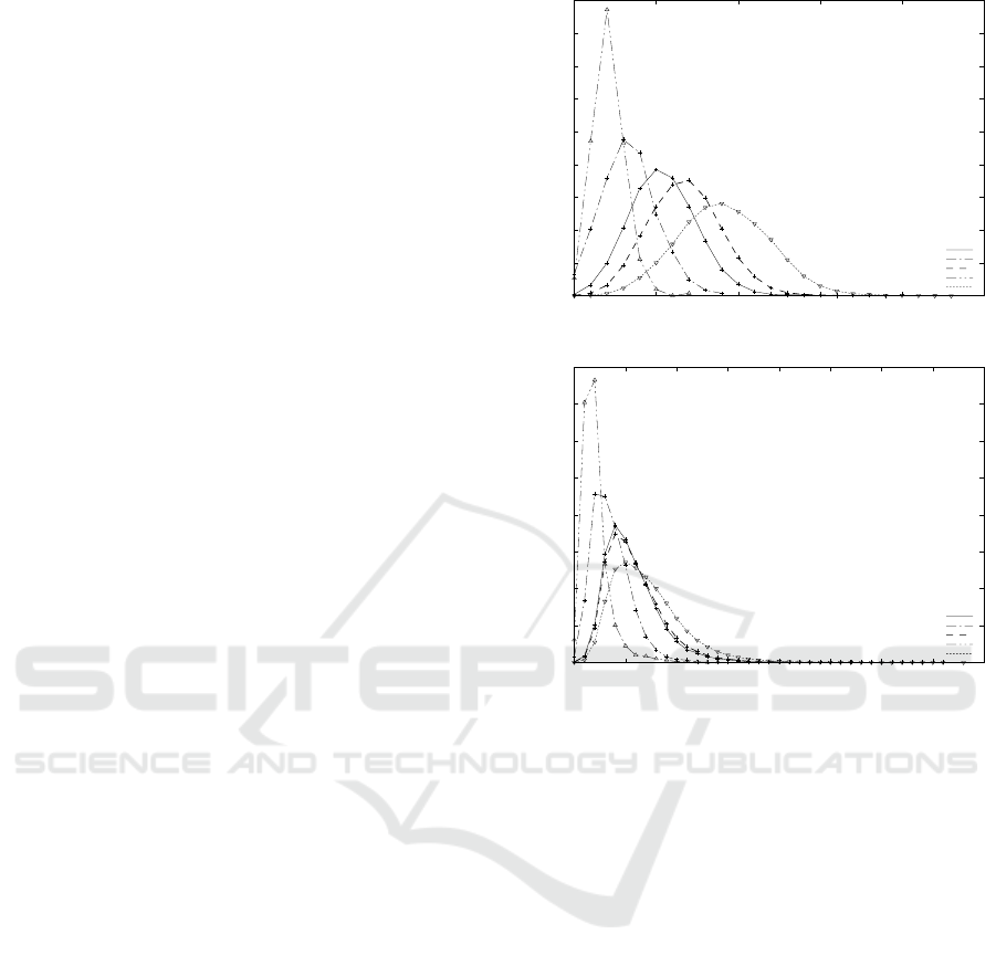
Table 3 shows that, as the experimental evaluation
of Theorem 5 (and 3), the running time of comput-
ing all the distances of d
V
, d
∗
V
, d
H
and d
∗
H
is much
smaller than that of the edit distance τ
TAI
, and the run-
ning time of computing the horizontal distance d
∗
H
is
smaller than that of the vertical distance d
∗
V
.
Note that, the reason why the running time of
computing d
V
for dblp
−
is extremely small is that the
height in every caterpillar in dblp
−
is either 1 or 2
and then the running time of σ(s(B
1
),s(B
2
)) is small.
Also, the height of 88% in caterpillars for CSLOGS is
from 1 to 3, which is the reason why the running time
of computingd
V
is smaller than that of other distances
for CSLOGS. Furthermore, in contrast to Theorem 5,
the running time of computing d
V
and d
∗
V
(in O(h
2
)
and O(h
2
+ λ) time in theoretical) is not much larger
than that of d
H
and hd
∗
(in O(λ) and O(λ + h) time
in theoretical), because we conjecture that the height
in caterpillars for all the data is too small to influence
the running time.
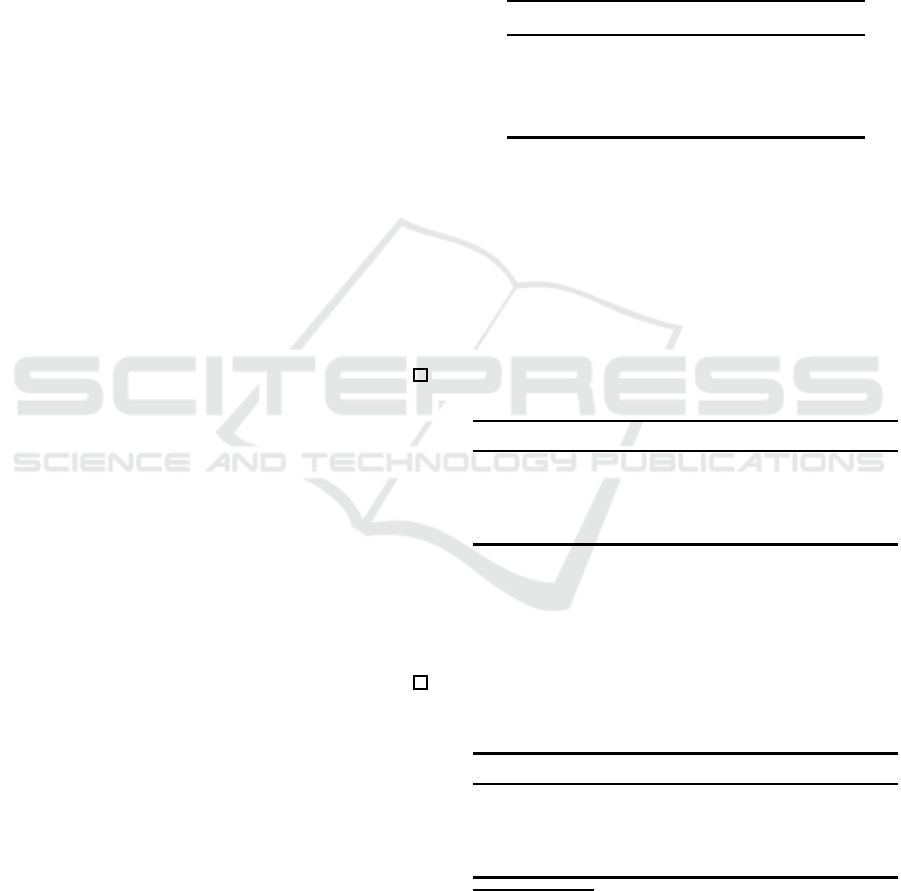
Next, we compare the distances of d
V
, d
∗
V
, d
H
, d
∗
H
and τ
TAI
. Figure 2 illustrates the distributions of the
distances for N-glycans and all-glycans. Also Fig-
ure 3 and 4 illustrate the distributions of the distances
to 10, from 10 to 30, from 30 to 100 and from 100,
for CSLOGS and dblp
−
, respectively. Since we can-
not compute τ
TAI
for CSLOGS, Figure 3 presents the
distances of d
V
, d
∗
V
, d
H
and d
∗
H
. Since the vertical
distance d
V
for more than 99% pairs of caterpillars in
CSLOGS is 0 or 1, Figure 4 presents the distances of
d
∗
V
, d
H
, d
∗
H
and τ
TAI
Figure 2 shows that the forms of all the distribu-
tions in are nearly normal, lbd is left to τ
TAI
and τ
TAI
is left to ubd. On the other hand, Figure 3 and 4 show
that the forms of distributions are not normal, but con-
centrate small values. Figure 3 shows that more than
90% pairs of caterpillars for CSLOGS concentrate on
the distances within 30, where the maximum values of
d
V
, d
∗
V
, d
H
and d
∗
H
are 70, 579, 403 and 473, respec-
tively. Also Figure 4 shows that more than 90% pairs
of caterpillars for dblp
−
concentrate on the distances
within 40, where the maximum values of τ
TAI
. d
∗
V
, d
H
and d
∗
H
are 746, 813, 745 and 746, respectively.
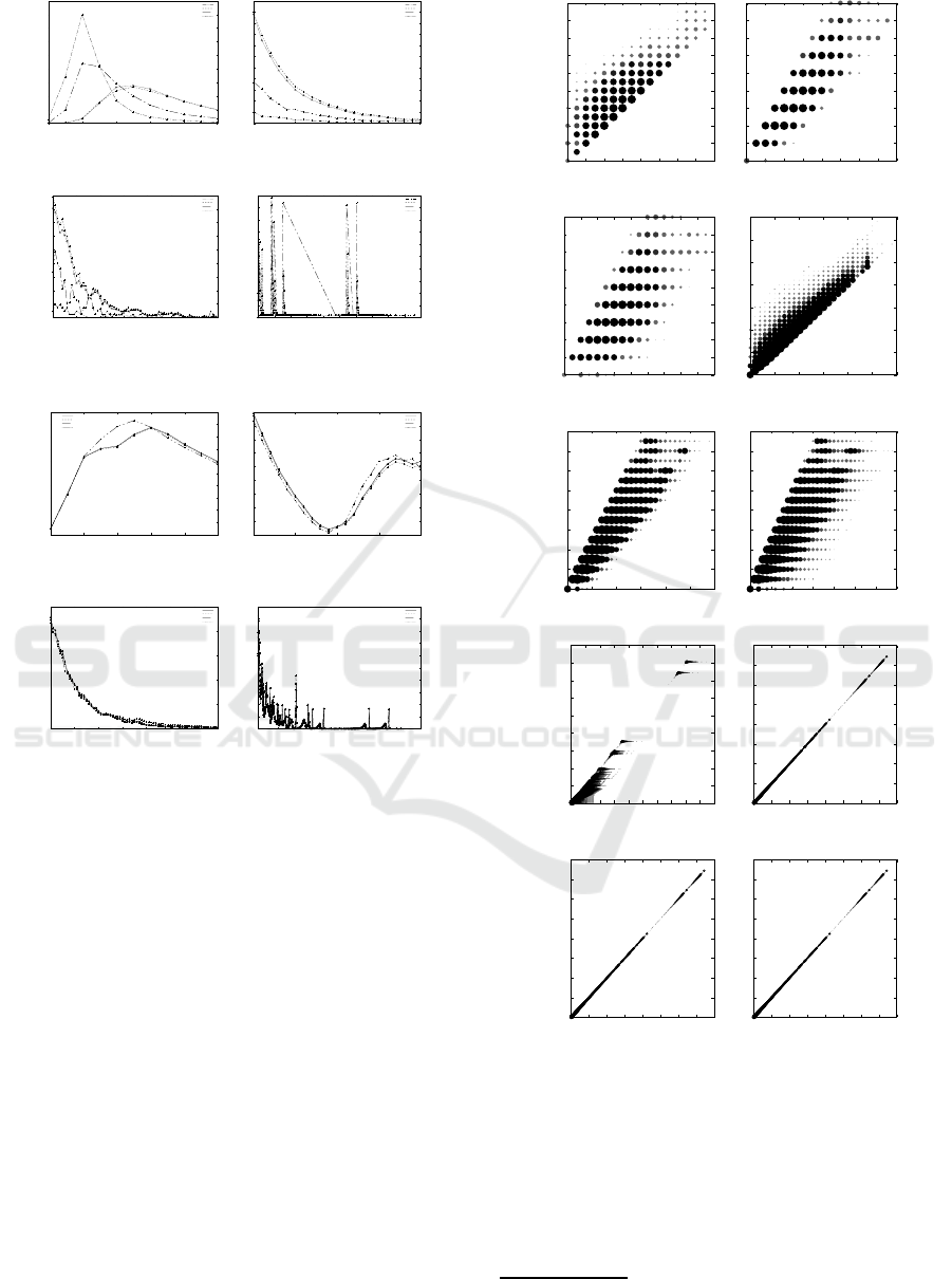
Figure 5 illustrates the scatter charts of lbd, ubd
and τ
TAI
for N-glycans, all-glycans, CSLOGS and
dblp
−
. Here, the representation of d
y
/d
x
means that
the number of pairs of caterpillars with the distance
d
x
is pointed at the x-axis and that with the distance
d
y
at the y-axis.
Since the number of caterpillars in N-glycans is
small, so the scatter charts in Figure 5 are sparse. For
N-glycans and all-glycans, the difference between a
pair of ubd, lbd and τ
TAI
is almost within 10. For
CSLOGS and dblp
−
, the difference is not large.
0
0.05
0.1
0.15
0.2
0.25
0.3
0.35
0.4
0.45
0 5 10 15 20 25
%
distance
edit distance
d
V
d
V
*
d
H
d
H
*
N-glycans
0
0.05
0.1
0.15
0.2
0.25
0.3
0.35
0.4
0 5 10 15 20 25 30 35 40
%
distance
TAI
d
V
d
V
*
d
H
d
H
*
all-glycans
Figure 2: The distributions of distances for N-glycans and
all-glycans.
In order to cofirm it in more detail, we evaluate
how the lower bound distances and the upper bound
distances approximate to the edit distance. Then, Ta-
ble 4 illustrates the difference diff for N-glycans, all-
glycans, dblp
−
and CSLOGS.
Table 4 shows that more than 93% of caterpillars
for N-glycans satisfy that diff ≤ 5, more than 94% of
caterpillars for all-glycans satisfy that diff ≤ 4, more
than 99% of caterpillars for dblp
−
satisfy that diff ≤ 1
and more than 92% of caterpillars for CSLOGS sat-
isfy that diff ≤ 5.
Hence, since more than 90% (resp., 98%) of cater-
pillars satisfy that diff ≤ 5 (resp., diff ≤ 10), we can
conclude that max{d
V
,d
H
} and min{d
∗
V
,d
∗
H
} succeed
to approximate τ
TAI
within 5 (resp., 10). This result is
important for the case that the running time of com-
puting τ
TAI
is large as CSLOGS.
Vertical and Horizontal Distances to Approximate Edit Distance for Rooted Labeled Caterpillars
595
0
0.05
0.1
0.15
0.2
0.25
0.3
0.35
0.4
0.45
0 2 4 6 8 10
%
distance
d
V
d
V
*
d
H
d
H
*
0
0.005
0.01
0.015
0.02
0.025
0.03
0.035
0.04
0.045
0.05
0.055
10 15 20 25 30
%
distance
d
V
d
V
*
d
H
d
H
*
d ≤ 10 10 ≤ d ≤ 30
0
0.0002
0.0004
0.0006
0.0008
0.001
0.0012
0.0014
0.0016
0.0018
30 40 50 60 70 80 90 100
%
distance
d
V
d
V
*
d
H
d
H
*
0
5×10
−6
1×10
−5
1.5×10
−5
2×10
−5
2.5×10
−5
3×10
−5
3.5×10
−5
4×10
−5
4.5×10
−5
5×10
−5
100 150 200 250 300 350 400 450 500 550 600
%
distance
d
V
d
V
*
d
H
d
H
*
30 ≤ d ≤ 100 d ≥ 100
Figure 3: The distributions of distances for CSLOGS.
0
0.005
0.01
0.015
0.02
0.025
0.03
0.035
0.04
0.045
0.05
0 2 4 6 8 10
%
distance
TAI
d
V
*
d
H
d
H
*
0.012
0.014
0.016
0.018
0.02
0.022
0.024
0.026
0.028
0.03
10 15 20 25 30
%
distance
TAI
d
V
*
d
H
d
H
*
d ≤ 10 10 ≤ d ≤ 30
0
0.005
0.01
0.015
0.02
0.025
30 40 50 60 70 80 90 100
%
distance
TAI
d
V
*
d
H
d
H
*
0
5×10
−5
0.0001
0.00015
0.0002
0.00025
0.0003
0.00035
0.0004
0.00045
0.0005
100 200 300 400 500 600 700 800 900
%
distance
TAI
d
V
*
d
H
d
H
*
30 ≤ d ≤ 100 d ≥ 100
Figure 4: The distributions of distances for dblp
−
.
5 CONCLUSION
In this paper, we have formulated the vertical dis-
tances d
V
and d
∗
V
and the horizontal distances d
H
and
d
∗
H
to approximate the edit distance τ
TAI
. Then, we
have shown the following inequality:
max{d
V
,d
H
} ≤ τ
TAI
≤ min{d
∗
V
,d
∗
H
}.
Furthermore, we have shown that, if we adopt the
unit cost function, then we can compute d
V
and d
∗
V
in quadratic time and d
H
and d
∗
H
in linear time.
Finally, we have given the experimental results to
evaluate the inequality and the running time for N-
glycans, all-glycans, CSLOGS and dblp
−
. Then, we
can conclude that by combining d
V
, d
∗
V
, d
H
and d
∗
H
,
we can approximate to the edit distance well such that
min{d
∗
V
,d
∗
H
} − max{d
V
,d
H
} ≤ 5
for more than 90% of caterpillars.
It is a future work to give experimental results
for other data such as SwissProt, TPC-H, Auction,
0
2
4
6
8
10
12
14
16
18
0 2 4 6 8 10 12 14 16
MIN
TAI
0
1
2
3
4
5
6
7
8
9
0 2 4 6 8 10 12 14 16
MAX
TAI
lbd/τ
TAI
, N-glycans ubd/τ
TAI
, N-glycans
0
1
2
3
4
5
6
7
8
9
0 2 4 6 8 10 12 14 16 18
MAX
MIN
0
5
10
15
20
25
30
35
0 5 10 15 20 25 30
MIN
TAI
lbd/ubd, N-glycans lbd/τ
TAI
, all-glycans
0
2
4
6
8
10
12
14
16
0 5 10 15 20 25 30
MAX
TAI
0
2
4
6
8
10
12
14
16
0 5 10 15 20 25 30 35
MAX
MIN
ubd/τ
TAI
, all-glycans lbd/ubd, all-glycans
0
50
100
150
200
250
300
350
400
450
0 50 100 150 200 250 300 350 400 450 500
MAX
MIN
0
100
200
300
400
500
600
700
800
0 100 200 300 400 500 600 700 800
MAX
TAI
lbd/ubd, CSLOGS lbd/τ
TAI
, dblp
−
0
100
200
300
400
500
600
700
800
0 100 200 300 400 500 600 700 800
MAX
TAI
0
100
200
300
400
500
600
700
800
0 100 200 300 400 500 600 700 800
MAX
TAI
ubd/τ
TAI
, dblp
−
lbd/ubd, dblp
−
Figure 5: The scatter charts of of lbd, ubd and τ
TAI
for N-
glycans, all-glycans, CSLOGS and dblp
−
.
University, Protein and Nasa from UW XML Reposi-
tory
4
. Note that, whereas the last four data contain no
caterpillars, we can obtain many caterpillars by delet-
ing the root (cf., (Muraka et al., 2018)).
4
UW XML Repository, http://aiweb.cs.washington.edu
/research/projects/xmltk/xmldata/www/repository.html
ICPRAM 2019 - 8th International Conference on Pattern Recognition Applications and Methods
596

Table 4: The difference diff for N-glycans, all-glycans,
dblp
−
and CSLOGS.
N-glycans
diff # %
0 2,448 1.86
1 17,091 12.96
2 32,404 24.58
3 33,949 25.75
4 24,240 18.46
5 13,420 10.18
6 5,801 4.40
7 1,751 1.33
8 475 0.36
9 109 0.08
10 47 0.04
11 6 0.00
dblp
−
diff # %
0 6,960,854 52.42
1 6,198,038 46.67
2 119,889 0.90
3 500 0.00
all-glycans
diff # %
0 1,105,515 3.47
1 11,619,644 34.46
2 10,547,139 33.10
3 4,633,275 14.54
4 2,108,501 6.62
5 1,001,311 3.14
6 458,637 1.44
7 203,334 0.64
8 110,184 0.35
9 49,385 0.16
10 20,461 0.06
11 6,999 0.02
12 2,393 0.01
13 801 0.00
14 350 0.00
15 147 0.00
16 30 0.00
17 18 0.00
18 8 0.00
19 3 0.00
20 1 0.00
CSLOGS
diff # %
0 10,513,132 1.22
1 174,777,470 20.21
2 301,960,142 34.91
3 175,761,327 20.32
4 90,141,737 10.42
5 42,955,474 4.97
6 23,342,365 2.70
7 14,094,693 1.63
diff # %
8 8,791,664 1.02
9 5,472,715 0.63
10 3,612,677 0.42
11 2,667,528 0.31
12 2,046,998 0.24
13 1,567,370 0.18
14 1,247,637 0.14
≥ 15 5,973,407 0.69
One of the reason that the approximation suc-
ceeds is that every node in a caterpillar is either an
element of the backbone or a leaf, that is, V(C) =
bb(C) ∪ lv(C). Also d
V
and d
∗
V
are based on a string
edit distance for bb(C) and d
H
and d
∗
H
are based on
a multiset edit distance for lv(C). When we can ex-
tend these distances to standard trees, it is necessary
how to determine a backbone and to deal with internal
nodes, which is a future work.
Concerned with the horizontal distances, we can
consider the repetition of the bag distance between
leaves after removing leaves from trees as possible.
Then, it is a future work to analyze such a distance.
ACKNOWLEDGMENTS
This work is partially supported by Grant-in-Aid
for Scientific Research 17H00762, 16H02870 and
16H01743 from the Ministry of Education, Culture,
Sports, Science and Technology, Japan.
REFERENCES
Akutsu, T., Fukagawa, D., Halld´orsson, M. M., Takasu, A.,
and Tanaka, K. (2013). Approximation and parame-
terized algorithms for common subtrees and edit dis-
tance between unordered trees. Theoret. Comput. Sci.,
470:10–22.
Deza, M. M. and Deza, E. (2016). Encyclopedia of dis-
tances (4th ed.). Springer.
Gallian, J. A. (2007). A dynamic survey of graph labeling.
Electorn. J. Combin., 14:DS6.
Hirata, K., Yamamoto, Y., and Kuboyama, T. (2011). Im-
proved MAX SNP-hard results for finding an edit dis-
tance between unordered trees. In Proc. CPM’11
(LNCS 6661), pages 402–415.
Kawaguchi, T., Yoshino, T., and Hirata, K. (2018). Path
histogram distance for rooted labeled caterpillars. In
Proc. ACIIDS’18 (LNAI 10751), pages 276–286.
Muraka, K., Yoshino, T., and Hirata, K. (2018). Computing
edit distance between rooted labeled caterpillars. In
Proc. FedCSIS’18, pages 245–252.
Tai, K.-C. (1979). The tree-to-tree correction problem. J.
ACM, 26:422–433.
Yamamoto, Y., Hirata, K., and Kuboyama, T. (2014).
Tractable and intractable variations of unordered tree
edit distance. Internat. J. Found. Comput. Sci.,
25:307–329.
Yoshino, T., Muraka, K., and Hirata, K. (2018). LCA his-
togram distance for rooted labeled caterpillars. In
Proc. KDIR’18, pages 307–314.
Zhang, K. and Jiang, T. (1994). Some MAX SNP-hard re-
sults concerning unordered labeled trees. Inform. Pro-
cess. Lett., 49:249–254.
Zhang, K., Wang, J., and Shasha, D. (1996). On the editing
distance between undirected acyclic graphs. Internat.
J. Found. Comput. Sci., 7:43–58.
Vertical and Horizontal Distances to Approximate Edit Distance for Rooted Labeled Caterpillars
597
