Faster RBF Network Learning Utilizing Singular Regions
Seiya Satoh
1
and Ryohei Nakano
2
1
Tokyo Denki University, Ishizaka, Hatoyama-machi, Hiki-gun, Saitama 350-0394, Japan
2
Chubu University, 1200 Matsumoto-cho, Kasugai, 487-8501, Japan
Keywords:
Neural Networks, RBF Networks, Learning Method, Singular Region, Reducibility Mapping.
Abstract:
There are two ways to learn radial basis function (RBF) networks: one-stage and two-stage learnings. Recently
a very powerful one-stage learning method called RBF-SSF has been proposed, which can stably find a series
of excellent solutions, making good use of singular regions, and can monotonically decrease training error
along with the increase of hidden units. RBF-SSF was built by applying the SSF (singularity stairs following)
paradigm to RBF networks; the SSF paradigm was originally and successfully proposed for multilayer percep-
trons. Although RBF-SSF has the strong capability to find excellent solutions, it required a lot of time mainly
because it computes the Hessian. This paper proposes a faster version of RBF-SSF called RBF-SSF(pH) by
introducing partial calculation of the Hessian. The experiments using two datasets showed RBF-SSF(pH) ran
as fast as usual one-stage learning methods while keeping the excellent solution quality.
1 INTRODUCTION
A radial basis function (RBF) network has the capa-
bility of universal approximation and is a popular al-
ternative to a multilayer perceptron (MLP). An RBF
network has the following parameters to learn: RBF
centers (composed of weights between input and hid-
den layers), their widths such as variances in Gaus-
sian basis functions, and weights between hidden and
output layers.
So far, many methods have been proposed to learn
RBF networks (Wu et al., 2012), and most methods
can be classified into two kinds: one-stage and two-
stage learnings. One-stage learning optimizes all the
parameters at the same time by using gradient-based
methods or the EM algorithm (Dempster et al., 1977).
On the other hand, Two-stage learning goes in two
stages; first, it selects suitable RBF centers together
with their widths, and then optimizes only the remain-
ing weights by solving linear regressions. (Bishop,
1995). Two-stage learning runs very fast and has been
very popular. Although one-stage learning requires
much more processing time than two-stage learning,
it finds solutions having smaller training errors than
two-stage learning for the same model complexity
(Satoh and Nakano, 2018). Incidentally, three-stage
learning has been investigated for classification task
(Schwenker et al., 2001).
Recently a very powerful one-stage learning
method called RBF-SSF has been proposed (Satoh
and Nakano, 2018), which can stably find a series of
excellent solutions, making good use of singular re-
gions, and can monotonically decrease training error
along with the increase of hidden units. RBF-SSF is
built by applying the SSF (singularity stairs follow-
ing) paradigm to RBF networks; the SSF paradigm
was originally proposed for MLPs with great suc-
cess (Satoh and Nakano, 2013) (Satoh and Nakano,
2015). Although RBF-SSF has the strong capability
to find excellent solutions, it required a lot of process-
ing time, even longer than a usual one-stage learning
method mainly because it computes the Hessian.
This paper proposes a faster version of RBF-SSF
called RBF-SSF(pH) by introducing partial calcula-
tion of the Hessian matrix, and compares its perfor-
mance with those of the original RBF-SSF, a typical
two-stage learning method, and usual one-stage learn-
ing methods.
This paper is organized as follows. Section 2
reviews RBF network formalization, existing learn-
ing methods, and singular regions as the background
knowledge. Section 3 proposes RBF-SSF(pH), ex-
plaining a general flow, partial Hessian calculation,
and other techniques for making SSF faster. Section
4 describes our experiments evaluating the solution
quality and processing time of RBF-SSF(pH) in com-
parison with the original RBF-SSF and three existing
methods. Section 5 summarizes the paper.
Satoh, S. and Nakano, R.
Faster RBF Network Learning Utilizing Singular Regions.
DOI: 10.5220/0007367205010508
In Proceedings of the 8th International Conference on Pattern Recognition Applications and Methods (ICPRAM 2019), pages 501-508
ISBN: 978-989-758-351-3
Copyright
c
 2019 by SCITEPRESS – Science and Technology Publications, Lda. All rights reserved
501

2 BACKGROUND
2.1 RBF Networks
Let RBF(J) be an RBF network with J hidden units
and one output unit. In RBF(J) model, let w
(J)
j
=
(w
(J)
j1
,··· , w
(J)
jK
)
T
be a vector of weights between all
input units and hidden unit j (= 1,··· ,J), and let v
(J)
j
be a weight between hidden unit j (= 0,1,··· ,J) and
a single output unit. When Gaussian basis function
is adopted and µ-th data point x
µ
= (x
µ
1
,··· , x
µ
K
)
T
is
given as input, the output of RBF(J) can be defined
as below. Here σ
j
is a width parameter of Gaussian
basis function at hidden unit j.
f
µ
J
= v
(J)
0
+
J
∑
j=1
v
(J)
j
exp


−
||x
µ
−w
(J)
j
||
2
2(σ
(J)
j
)
2


(1)
The whole parameter vector of RBF(J) is given as be-
low:
θ
(J)
=

v
(J)
0
,··· , v
(J)
J
,

w
(J)
1

T
,··· ,

w
(J)
J

T
,
σ
(J)
1
,··· ,σ
(J)
J

T
. (2)
Given training data {(x
µ
,y
µ
), µ = 1,··· ,N}, the target
function of RBF(J) learning is given as follows.
E
J
=
1
2
N
∑
µ=1

δ
µ
J

2
, δ
µ
J
≡ f
µ
J
−y
µ
(3)
2.2 Existing RBF Network Learning
Methods
Many methods to learn RBF networks can be classi-
fied into two kinds: one-stage learning and two-stage
learning.
In one-stage learning, whole weights are opti-
mized at the same time by using gradient-based meth-
ods or the EM algorithm (Dempster et al., 1977).
Gradient-based methods can be classified into 1st-
order methods such as the steepest descent and 2nd-
order methods such as quasi-Newton method.
In two-stage learning, under the condition that
σ
(J)
1
,···,σ
(J)
J
are fixed to a certain constant throughout
learning, first, select suitable w
(J)
1
,··· , w
(J)
J
, and then,
optimize v
(J)
0
,··· ,v
(J)
J
by solving linear regressions
(Bishop, 1995).
One-stage Learning
One-stage learning can be classified into gradient-
based or mixture-based (L´azaro et al., 2003). In the
following experiments, we employ steepest descent
(SD) as a 1st-order method and BFGS (quasi-Newton
method with the BFGS update) (Fletcher, 1987) as a
2nd-order method.
Two-stage Learning
At the first stage of this learning, one can apply clus-
tering to explanatory data {x
µ
} to get J clusters, and
then treat all the centroids as w
(J)
1
,··· , w
(J)
J
.
This paper, however, employs function newrb
available in Neural Network Toolbox of MATLAB
R2015b. The newrb algorithm gradually expands an
RBF network by increasing the number J of hidden
units one by one. At each cycle of model expansion,
data point x
µ
that has the largest value of output error
|f
µ
J−1
−y
µ
| is added as w
J
. Width parameters {σ
j
} of
basis functions are not optimized in this learning.
The general flow of the newrb algorithm is shown
below. Let J
max
be the maximum number of hidden
units.
Algorithm 1: Newrb algorithm.
1: v
0
← (1/N)
∑
N
µ=1
y
µ
2: for J = 1,··· ,J
max
do
3: Compute outputs f
µ
J−1
, µ = 1,··· ,N.
4: i ←argmax
µ∈{1,···,N}
|f
µ
J−1
−y
µ
|
5: w
(J)
J
← x
i
6: With w
(J)
1
,··· , w
(J)
J
fixed, optimize
v
(J)
0
,··· , v
(J)
J
.
7: end for
2.3 Singular Regions of RBF Networks
The search space of MLP has a continuous region
where input-output equivalence holds and the gradi-
ent is zero (Fukumizu and Amari, 2000) (Nitta, 2013).
Such regions can be generated by using reducibility
mapping αβ or γ (Satoh and Nakano, 2013) (Satoh
and Nakano, 2015). We call such a region a singular
region.
The search space of an RBF network has also sin-
gular regions, which are generated only by reducibil-
ity mapping γ.
Below we explain how to generate a singular re-
gion of RBF(J) based on the optimal solution of
RBF(J−1). The optimal solution must satisfy the
following, where E
J−1
denotes the target function of
RBF(J−1) learning, and θ
(J−1)
denotes the whole pa-
rameter vector of RBF(J−1).
∂E
J−1
∂θ
(J−1)
= 0 (4)
ICPRAM 2019 - 8th International Conference on Pattern Recognition Applications and Methods
502

This can be broken down element-wise as follows,
where j = 1,···, J −1.
∂E
J−1
∂v
(J−1)
0
=
N
∑
µ=1
δ
µ
J−1
= 0 (5)
∂E
J−1
∂v
(J−1)
j
=
∑
µ
δ
µ
J−1
exp


−
||x
µ
−w
(J−1)
j
||
2
2(σ
(J−1)
j
)
2


=0 (6)
∂E
J−1
∂w
(J−1)
j
=
∑
µ
δ
µ
J−1
v
(J−1)
j
exp


−
||x
µ
−w
(J−1)
j
||
2
2(σ
(J−1)
j
)
2


x
µ
−w
(J−1)
j

σ
(J−1)
j

2
= 0 (7)
∂E
J−1
∂σ
(J−1)
j
=
∑
µ
δ
µ
J−1
v
(J−1)
j
exp


−
||x
µ
−w
(J−1)
j
||
2
2(σ
(J−1)
j
)
2


||x
µ
−w
(J−1)
j
||
2

σ
(J−1)
j

3
= 0 (8)
Let the optimal solution
b
θ
(J−1)
of RBF(J−1) be

bv
(J−1)
0
,··· , bv
(J−1)
J
,

b
w
(J−1)
1

T
,··· ,

b
w
(J−1)
J

T
,
b
σ
(J−1)
1
,··· ,
b
σ
(J−1)
J

T
.
Now apply reducibility mapping γ to the optimal so-
lution
b
θ
(J−1)
to get singular region
b
Θ
(J)
γ
. Here m ∈
{1,···, J −1}.
b
θ
(J−1)
γ
−→
b
Θ
(J)
γ
b
Θ
(J)
γ
≡ {θ
(J)
| v
(J)
0
= bv
(J−1)
0
,v
(J)
m
+ v
(J)
J
= bv
(J−1)
m
,
w
(J)
m
= w
(J)
J
=
b
w
(J−1)
m
,σ
(J)
m
= σ
(J)
J
=
b
σ
(J−1)
m
,
v
(J)
j
= bv
(J−1)
j
,w
(J)
j
=
b
w
(J−1)
j
,σ
(J)
j
=
b
σ
(J−1)
j
,
for j ∈ {1,···, J −1}\{m}} (9)
Note that v
(J)
m
and v
(J)
J
cannot be determined uniquely
since they only have the following constraint.
v
(J)
m
+ v
(J)
J
= bv
(J−1)
m
(10)
This equation can be rewritten using the following q.
v
(J)
m
= q bv
(J−1)
m
, v
(J)
J
= (1−q) bv
(J−1)
m
(11)
3 RBF-SSF(pH)
A search paradigm called Singularity Stairs Follow-
ing (SSF) stably finds a series of excellent solutions
by making good use of singular regions.
For MLPs two series of SSF methods have been
proposed: the latest versions are SSF1.4 (Satoh and
Nakano, 2013) for real-valued MLPs and C-SSF1.3
(Satoh and Nakano, 2015) for complex-valuedMLPs.
By applying the SSF paradigm to RBF networks,
RBF-SSF has been proposed (Satoh and Nakano,
2018). Although RBF-SSF stably finds excellent so-
lutions having much simpler model complexities and
much smaller training errors, it takes a lot of process-
ing time. Its processing time is longer than a usual
one-stage learning method such as steepest descent or
BFGS (quasi-Newton with the BFGS update).
Since RBF-SSF employs BFGS as its basic search
engine, the difference comes from whether to calcu-
late the Hessian or not. Any SSF calculates the Hes-
sian at its starting from a singular region to find search
directions because the gradient is zero in a singular
region. Note that the eigenvector corresponding to
a negative eigenvalue of the Hessian indicates a de-
scending direction from the singular region.
Thus, one way to make RBF-SSF much faster is
to drastically reduce the calculation time of the Hes-
sian. For this reason we introduce calculating the
partial Hessian instead of the full Hessian. The full
Hessian is a square matrix of size M
f
, the number of
all the parameters; M
f
= J(K + 2) + 1. On the other
hand, the partial Hessian is a square matrix of size
M
p
= 2(K + 2) + 1. When J gets large, calculation
time of the full Hessian increases in the order of J
2
,
while that of the partial Hessian remains a small con-
stant. Note that RBF-SSF optimizes {σ
j
} as well.
3.1 General Flow of RBF-SSF(pH)
The general flow of RBF-SSF(pH) is shown below.
Let J
max
be the maximum number of hidden units.
Algorithm 2: General flow of RBF-SSF(pH.
1: Get the best solution of RBF(J =1) by repeating
search with different initial weights.
2: for J = 2,··· ,J
max
do
3: Select starting points from the singular region
obtained by applying reducibility mapping γ to
the best solution of RBF(J−1).
4: Calculate partial Hessian at each starting point,
calculate eigenvalues and eigenvectors of the
partial Hessian, and select eigenvectors corre-
sponding to each negative eigenvalue.
5: Repeat search predefined times from the start-
ing points in the direction and in the opposite
direction of an eigenvector selected at Step 4,
and get the best solution of RBF(J).
6: end for
Faster RBF Network Learning Utilizing Singular Regions
503

In the following experiments, the starting points
from a singular region at the aboveStep 3 are obtained
by setting q to 0.5,1.0, and 1.5 in eq.(11). These
three points correspond to interpolation, boundary,
and extrapolation. Since m is changed in the range
of 1,··· ,J −1, the total number of starting points in
the search of RBF(J) amounts to 3(J −1).
3.2 Calculation of the Partial Hessian
The Hessian matrix is a symmetric matrix of second
derivatives of the target function. Although the first
derivatives are easy to calculate, second derivatives
require complicated and heavy calculation.
The partial Hessian is shown below. Although the
full Hessian is composed of 2nd derivatives with re-
spect to all the parameters θ
(J)
shown in eq.(2), the
partial Hessian is limited to m and J.
∂
2
E
J
∂θ
(J)
m,J
∂θ
(J)
m,J
T
(12)
Here
θ
(J)
m,J
≡

v
(J)
0
,v
(J)
m
,v
(J)
J
,

w
(J)
m

T
,

w
(J)
J

T
,σ
(J)
m
,σ
(J)
J

T
. (13)
The number of elements of the full Hessian is
M
2
f
= (J(K + 2) + 1)
2
, while that of the partial Hes-
sian is M
2
p
= (2(K + 2) + 1)
2
. Since the Hessian
is symmetric, the actual number of elements to cal-
culate is M
f
(M
f
+ 1)/2 for the full Hessian, and
M
p
(M
p
+ 1)/2 for the partial Hessian.
3.3 Other Techniques for Making
SSF-SSFs Faster
The section explains the techniques for making SSF
for MLPS faster (Satoh and Nakano, 2015), which
can be applied to RBF-SSF and RBF-SSF(pH).
The number of starting points of RBF(J) gets large
as J gets large. Moreover, the dimension of the search
space also gets large as J gets large. Thus, if we per-
form search for every negative eigenvalue for large
J, the number of searches gets very large, and con-
sequently the processing time becomes huge. Hence,
we introduce two accelerating techniques into RBF-
SSF: one is search pruning and the other is to set up-
per limit to the number of searches.
Search pruning is an accelerating technique which
discards a search if the search is found to proceed
along much the same route experienced before (Satoh
and Nakano, 2013).
Setting upper limit to the number of searches is an
accelerating technique which selects the predefined
number of starting points based on the preference.
Here preference is given to smaller negative eigenval-
ues since such eigenvalues indicate bigger drop from
a search point. In the following experiments the upper
limit is set to be 10.
4 EXPERIMENTS
4.1 Design of Experiments
The performance of RBF-SSF(pH) was compared
with four other learning methods. Tabel 1 describes
these five methods. SD and BFGS are repeated 10
times changing initial weights. The number J of hid-
den units for newrb was changed as 10,20,···,500,
while J of SD, BFGS, RBF-SSF and RBF-SSF(pH)
was changed as 1,2, ··· ,50. Note that BFGS and two
RBF-SSFs adapt {σ
j
} through learning.
Table 1: Learning methods.
Learning Description
method
(j = 1,··· ,J)
newrb two-stage learning
σ
(J)
j
: fixed to be 1/
√
2
one-stage learning
batch steepest descent
with adaptive step length
SD the initial value of v
(J)
j
: 0
the initial value of w
(J)
j
:
randomly selected from {x
µ
}
σ
(J)
j
: fixed to be 1/
√
2
one-stage learning
quasi-Newton with BFGS update
BFGS the initial value of v
(J)
j
: 0
the initial value of w
(J)
j
:
randomly selected from {x
µ
}
the initial value of σ
(J)
j
: 1/
√
2
RBF-SSF one-stage learning by RBF-SSF
RBF-SSF(pH) faster version of RBF-SSF
We used the following two datasets: Schwe-
fel function dataset (Schwefel, 1981) and Parkin-
sons telemonitoring dataset from UCI ML Repository
(Dheeru and Taniskidou, 2017). Each dataset was
normalized as follows, where y
mean
and y
std
are the
average and standard deviation of {y
µ
} respectively.
ex
µ
k
←
x
µ
k
max
µ
(|x
µ
k
|)
, ey
µ
←
y
µ
−y
mean
y
std
(14)
ICPRAM 2019 - 8th International Conference on Pattern Recognition Applications and Methods
504

4.2 Experiments using Schwefel
Function Dataset
Schwefel function is given by eq.(15) (Schwefel,
1981). We set the function parameter K and the
ranges of variables x
k
as K = 2 and x
k
∈(−50, 50), and
then generated 2000 data points for training and other
2000 data points for test. Generated data were nor-
malized as shown above. After normalizing y
µ
, Gaus-
sian noise N (0,0.01
2
) was added for training data.
f(x
1
,..., x
K
) = 418.982887K−
K
∑
k=1
x
k
sin(
p
|x
k
|) (15)
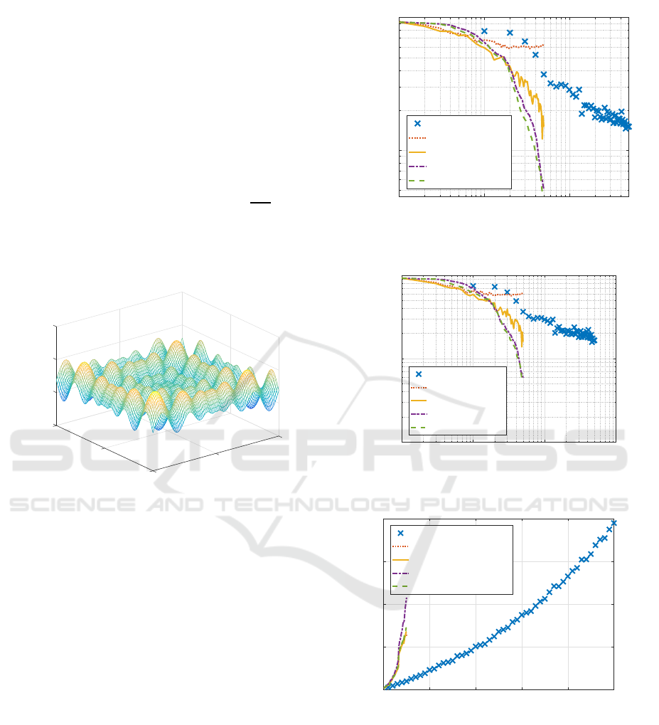
Figure 1 shows the generated function. We can
see this function has many peaks.
700
50
800
50
f
900
x
2
0
x
1
1000
0
-50
-50
Figure 1: Schwefel function (K = 2, x
1
,x
2
∈ (−50,50)).
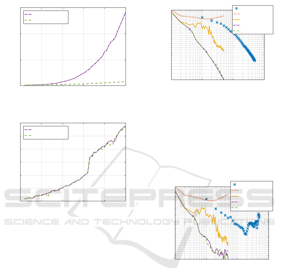
Figure 2 illustrates how five learning methods,
newrb, SD, BFGS, RBF-SSF, and RBF-SSF(pH), de-
creased training error with the increase of hidden
units for Schwefel function dataset. RBF-SSF(pH)
and RBF-SSF monotonically and sharply decreased
training error to the lowest, showing much the same
performance. BFGS and newrb could reach only
more than two times larger error than the lowest; note
that newrb used 10 times larger model complexity
than the others. Two RBF-SSFs and BFGS massively
outperformed newrb for any same model complexity.
SD hardly decreased training error.
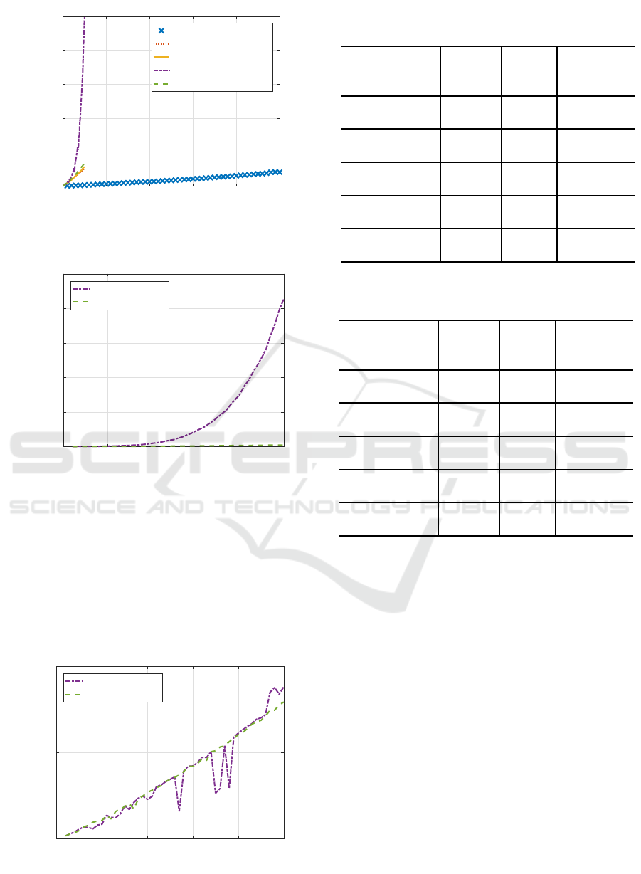
Figure 3 depicts test errors of five methods for
Schwefel function dataset. Two RBF-SSFs showed
much the same best performance. BFGS and newrb
decreased only to the level more than two times larger
test error than the best. Two RBF-SSFs and BFGS
outperformed newrb for each same model complex-
ity. SD hardly decreased test error.
Figure 4 shows total processing time of five meth-
ods for Schwefel function dataset. Newrb was the
fastest, while the rest four required more processing
10
0
10
1
10
2
Number of hidden units J
10
-1
10
0
MSE
training
newrb
SD
BFGS
RBF-SSF
RBF-SSF(pH)
Figure 2: Training error for Schwefel function dataset.
10
0
10
1
10
2
10
3
Number of hidden units J
10
-2
10
-1
10
0
MSE
test
newrb
SD
BFGS
RBF-SSF
RBF-SSF(pH)
Figure 3: Test error for Schwefel function dataset.
0 100 200 300 400 500
Number of hidden units J
0
20
40
60
80
Processing time (sec)
newrb (cumulative)
SD
BFGS
RBF-SSF
RBF-SSF(pH)
Figure 4: Total processing time for Schwefel function
dataset.
time. Among the four, only the original RBF-SSF re-
quired more processing time than the other three.
Figure 5 compares Hessian calculation time of
two RBF-SSFs. The figure clearly shows how Hes-
sian computation time was drastically reduced to a
small amount of time by the proposed RBF-SSF(pH)
compared with the original RBF-SSF.
Figure 6 shows the remaining processing time
Faster RBF Network Learning Utilizing Singular Regions
505

0 10 20 30 40 50
Number of hidden units J
0
5
10
15
Processing time (sec)
RBF-SSF
RBF-SSF(pH)
Figure 5: Processing time of Hessian calculation for Schwe-
fel function dataset.
0 10 20 30 40 50
Number of hidden units J
0
5
10
15
20
25
30
Processing time (sec)
RBF-SSF
RBF-SSF(pH)
Figure 6: Processing time of other calculations for Schwefel
function dataset.
other than Hessian calculation of two RBF-SSFs.
Two lines are closely overlapped, showing the rest
were much the same.
4.3 Experiments using Parkinsons
Telemonitoring Dataset
The problem for this dataset (Little et al., 2007) is to
estimate motor UPDRS (unified Parkinson’s disease
rating score) based on 18 explanatory variables such
as voice measures. The number N of data points is
5875; 90 % was used for training, and the remaining
10 % was used for test.
Figure 7 illustrates how five learning methods de-
creased training error for Parkinsons telemonitoring
dataset. Two RBF-SSFs monotonically and rapidly
decreased training error to the lowest, showing much
the same performance. Newrb and BFGS could reach
about 1.4 and 1.7 times larger error than the lowest re-
spectively. Note that again newrb used 10 times larger
model complexity than the others. Two RBF-SSFs
and BFGS significantly outperformed newrb for any
10
0
10
1
10
2
10
3
Number of hidden units J
0.3
0.4
0.5
0.6
0.7
0.8
0.9
MSE
training
newrb
SD
BFGS
RBF-SSF
RBF-SSF(pH)
Figure 7: Training error for Parkinsons telemonitoring
dataset.
same model complexity. SD hardly decreased train-
ing error.
Figure 8 depicts test errors of five methods for
Parkinsons telemonitoring dataset. Two RBF-SSFs
showed much the same best performance. BFGS and
newrb decreased test error to the level 1.2 and 1.3
times larger than the best. Two RBF-SSFs and BFGS
outperformed newrb for any same model complexity.
SD hardly decreased test error.
10
0
10
1
10
2
10
3
Number of hidden units J
0.4
0.45
0.5
0.55
0.6
0.65
0.7
0.75
0.8
0.85
0.9
MSE
test
newrb
SD
BFGS
RBF-SSF
RBF-SSF(pH)
Figure 8: Test error for Parkinsons telemonitoring dataset.
Figure 9 shows total processing time of five meth-
ods for Parkinsons telemonitoring dataset. Again
newrb was the fastest, the original RBF-SSF was the
slowest, and the remaining three required middle-
level processing time. The proposed RBF-SSF(pH)
ran slightly slower than SD and BFGS.
Figure 10 compares Hessian calculation time of
two RBF-SSFs. The figure clearly shows how Hes-
sian computation time was drastically reduced to a
negligible amount of time by the proposed RBF-
SSF(pH) compared with the original RBF-SSF.
Figure 11 shows the remaining processing time
other than Hessian calculation of two RBF-SSFs.
Two lines are mostly overlapped, showing the remain-
ing processing time was much the same.
ICPRAM 2019 - 8th International Conference on Pattern Recognition Applications and Methods
506

0 100 200 300 400 500
Number of hidden units J
0
1000
2000
3000
4000
5000
Processing time (sec)
newrb (cumulative)
SD
BFGS
RBF-SSF
RBF-SSF(pH)
Figure 9: Total processing time for Parkinsons telemonitor-
ing dataset.
0 10 20 30 40 50
Number of hidden units J
0
1000
2000
3000
4000
5000
Processing time (sec)
RBF-SSF
RBF-SSF(pH)
Figure 10: Processing time of Hessian calculation for
Parkinsons telemonitoring dataset.
4.4 Comparison of Best Performances
Minimum training MSEs, minimum test MSEs, and
total processing time through all Js are shown in Ta-
bles 2 and 3. These two tables indicate the following.
(1) Minimum Training Errors
0 10 20 30 40 50
Number of hidden units J
0
200
400
600
800
Processing time (sec)
RBF-SSF
RBF-SSF(pH)
Figure 11: Processing time of other calculations for Parkin-
sons telemonitoring dataset.
Table 2: Performance comparison for Schwefel function
dataset.
min min total
learning
training test processing
method MSE MSE time (sec)
newrb 0.1456 0.1579 77.88
SD 0.5823 0.5659 546.93
BFGS 0.1212 0.1382 534.34
RBF-SSF 0.0505 0.0591 715.84
RBF-SSF(pH) 0.0449 0.0527 560.85
Table 3: Performance comparison for Parkinsons telemoni-
toring dataset.
min min total
learning
training test processing
method MSE MSE time (sec)
newrb 0.3558 0.5132 410
SD 0.7985 0.7609 12899
BFGS 0.4278 0.4496 13000
RBF-SSF 0.2463 0.3837 54902
RBF-SSF(pH) 0.2513 0.3834 15371
As for minimum training MSEs through all Js for
Schwefel function dataset, RBF-SSF(pH) achieved
the smallest, then RBF-SSF, BFGS, newrb, and SD
followed in ascending order, having 1.12, 2.70, 3.24,
and 13.0 times larger than the smallest respectively.
Note that newrb used 10 times larger model complex-
ities than the other methods.
For Parkinsons telemonitoring dataset, RBF-SSF
achieved the smallest, then RBF-SSF(pH), newrb,
BFGS, and SD followed in ascending order, having
1.02, 1.44, 1.74, and 3.24 times larger training MSEs
than the smallest respectively.
RBF-SSF(pH) and RBF-SSF obtained the com-
parable training MSEs, much smaller than those of
the other methods.
(2) Minimum Test Errors
As for minimum test MSEs through all Js for
Schwefel function dataset, RBF-SSF(pH) achieved
the smallest, then RBF-SSF, BFGS, newrb, and SD
followed in ascending order, having 1.12, 2.62, 3.00,
Faster RBF Network Learning Utilizing Singular Regions
507

and 10.7 times larger than the smallest respectively.
For Parkinsons telemonitoring dataset, RBF-
SSF(pH) and RBF-SSF achieved the smallest, then
BFGS, newrb, and SD followed in ascending order,
having 1.17, 1.34, and 1.98 times larger test MSEs
than the smallest respectively.
RBF-SSF(pH) and RBF-SSF obtained much the
same smallest test MSEs. Although a model having
too small training error often has rather poor test
error, suffering from overfitting, RBF-SSFs found
solutions having minimum training and test errors.
We think this is caused by the following; RBF-SSFs
have the strong capability to find excellent solutions,
and RBF networks are less prone to overfitting. We
do not think this is caused by small-noise datasets
because Parkinsons telemonitoring dataset has mini-
mum training MSE 0.25 and minimum test MSE 0.38
for normalized data.
(3) Total Processing Time
As for total processing time for Schwefel func-
tion dataset, newrb was the fastest since it just solved
linear regressions. Among the other four methods,
BFGS was the fastest, and then, SD, RBF-SSF(pH),
and RBF-SSF followed in order, requiring 1.02, 1.05,
and 1.34 times longer time than BFGS respectively.
For Parkinsons telemonitoring dataset, newrb was
the fastest, and among the other four, SD was the
fastest, and then, BFGS, RBF-SSF(pH), and RBF-
SSF followed in order, requiring 1.01, 1.19, and 4.26
times longer time than SD respectively.
The proposed RBF-SSF(pH) was 1.28 and 3.57
times faster than the original RBF-SSF, and was
1.05 and 1.18 times slower than BFGS. We can say
RBF-SSF(pH) runs almost as fast as a good learning
method BFGS. Moreover, to find excellent solutions
of RBF networks, some amount of processing time
will be needed.
5 CONCLUSIONS
Recently a very powerful one-stage learning method
RBF-SSF has been proposed to find excellent solu-
tions of RBF networks; however, it required a lot of
time mainly because it computes the Hessian. This
paper proposes a faster version of RBF-SSF called
RBF-SSF(pH) by introducing partial calculation of
the Hessian. The experiments using two datasets
showed RBF-SSF(pH) ran as fast as usual one-stage
learning methods while keeping the excellent solution
quality. In the future, we plan to apply RBF-SSF(pH)
to more data to prove its superiority.
ACKNOWLEDGMENT
This work was supported by Grants-in-Aid for Scien-
tific Research (C) 16K00342.
REFERENCES
Bishop, C. M. (1995). Neural networks for pattern recog-
nition. Oxford university press.
Dempster, A. P., Laird, N. M., and Rubin, D. B. (1977).
Maximum likelihood from incomplete data via the
EM algorithm. Journal of the royal statistical soci-
ety. Series B (methodological), 39:1–38.
Dheeru, D. and Taniskidou, E. K. (2017). UCI machine
learning repository.
Fletcher, R. (1987). Practical methods of optimization, 2nd
edition. JOHN WILEY & SONS.
Fukumizu, K. and Amari, S. (2000). Local minima and
plateaus in hierarchical structures of multilayer per-
ceptrons. Neural Networks, 13(3):317–327.
L´azaro, M., Santamarıa, I., and Pantale´on, C. (2003). A
new EM-based training algorithm for RBF networks.
Neural Networks, 16(1):69–77.
Little, M. A., McSharry, P. E., Roberts, S. J., Costello,
D. A., and Moroz, I. M. (2007). Exploiting nonlin-
ear recurrence and fractal scaling properties for voice
disorder detection. Biomedical Engineering Online,
6(1):23.
Nitta, T. (2013). Local minima in hierarchical structures of
complex-valued neural networks. Neural Networks,
43:1–7.
Satoh, S. and Nakano, R. (2013). Multilayer perceptron
learning utilizing singular regions and search pruning.
In Proc. Int. Conf. on Machine Learning and Data
Analysis, pages 790–795.
Satoh, S. and Nakano, R. (2015). A yet faster version
of complex-valued multilayer perceptron learning us-
ing singular regions and search pruning. In Proc.
of 7th Int. Joint Conf. on Computational Intelligence
(IJCCI), volume 3 NCTA, pages 122–129.
Satoh, S. and Nakano, R. (2018). A new method for learn-
ing RBF networks by utilizing singular regions. In
Proc. 17th Int. Conf. on Artificial Intelligence and Soft
Computing (ICAISC), pages 214–225.
Schwefel, H.-P. (1981). Numerical Optimization of Com-
puter Models. John Wiley & Sons, Inc.
Schwenker, F., Kestler, H. A., and Palm, G. (2001). Three
learning phases for radial-basis-function networks.
Neural networks, 14(4-5):439–458.
Wu, Y., Wang, H., Zhang, B., and Du, K.-L. (2012). Using
radial basis function networks for function approxi-
mation and classification. ISRN Applied Mathematics,
2012:1–34.
ICPRAM 2019 - 8th International Conference on Pattern Recognition Applications and Methods
508