
Band-limited Orthogonal Functional Systems
for Optical Fresnel Transform
Tomohiro Aoyagi, Kouichi Ohtsubo and Nobuo Aoyagi
Faculty of Information Sciences and Arts, Toyo University, 2100 Kujirai, Saitama, Japan
Keywords: Fresnel Transform, Dual Orthogonal Property, Eigenvalue Problem, Jacobi Method, Hermitian Matrix.
Abstract: The fundamental formula in an optical system is Rayleigh diffraction integral. In practice, we deal with
Fresnel diffraction integral as approximate diffraction formula. By optical instruments, an optical wave is
subject to a band limited. To reveal the band-limited effect in Fresnel transform plane, we seek the function
that its total power in finite Fresnel transform plane is maximized, on condition that an input signal is zero
outside the bounded region. This problem is a variational one with an accessory condition. This leads to the
eigenvalue problems of Fredholm integral equation of the first kind. The kernel of the integral equation is
Hermitian conjugate and positive definite. Therefore, eigenvalues are real non-negative numbers. Moreover,
we also prove that the eigenfunctions corresponding to distinct eigenvalues have dual orthogonal property.
By discretizing the kernel and integral calculus range, the eigenvalue problems of the integral equation depend
on a one of the Hermitian matrix in finite dimensional vector space. We use the Jacobi method to compute all
eigenvalues and eigenvectors of the matrix. We consider the application of the eigenvectors to the problem of
approximating a function and showed the validity of the eigenvectors in computer simulation.
1 INTRODUCTION
In scalar diffraction theory, the Huygens-Fresnel
principle is used to explain diffraction phenomenon.
The integral theorem of Helmholtz and Kirchhoff
plays an important role in the development of the
scalar theory of diffraction. Although scalar wave
propagation is fully described by a single scalar wave
equation, fundamental formula in an optical system is
Rayleigh diffraction integral. In practice, we deal
with Fresnel diffraction integral as approximate
diffraction formula. The Fresnel transform has been
studied mathematically and shown to be a one-
parameter group of unitary and factor-type operators
from its algebraic and topological properties in
Hilbert space (
) (Aoyagi, 1973, and Aoyagi et
al., 1973a). In recently, it is also used in image
processing, optical information processing, optical
waveguides, computer-generated holograms,
iterative phase retrieval techniques, speckle pattern
interferometry and so on. In optical applications, an
orthogonal functional system plays an important role.
Up to now, many orthogonal functional systems have
been derived in connection with the Fourier transform
and applied to many applications. The extension of
optical fields through an optical instrument is
practically limited to some finite area. By band-
limited effect in Fourier transform plane, sampling
functional systems have been derived and have
orthogonal property. From sampling theorem about
the Fourier transform, orthogonal functional systems
are formulated from the point of view of functional
analysis (Ogawa, 2009). In the literature, there are
many sampling theorems and examples about the
Fourier transform. Its applications and references
therein (Jerri, 1977). However, the property of the
orthogonal function about Fresnel transform is not
revealed sufficiently.
In this paper, the band-limited effect in Fresnel
transform plane is investigated. For that, we seek the
function that its total power in finite Fresnel
transform plane is maximized, on condition that an
input signal is zero outside the bounded region. This
problem is a variational one with an accessory
condition. This leads to the eigenvalue problems of
Fredholm integral equation of the first kind (Kondo,
1954). The kernel of the integral equation is
Hermitian conjugate and positive definite. Therefore,
eigenvalues are real non-negative numbers.
Moreover, we prove that the eigenfunctions
corresponding to distinct eigenvalues have dual
orthogonal property. By discretizing the kernel and
Aoyagi, T., Ohtsubo, K. and Aoyagi, N.
Band-limited Orthogonal Functional Systems for Optical Fresnel Transform.
DOI: 10.5220/0007367001470153
In Proceedings of the 7th International Conference on Photonics, Optics and Laser Technology (PHOTOPTICS 2019), pages 147-153
ISBN: 978-989-758-364-3
Copyright
c
2019 by SCITEPRESS – Science and Technology Publications, Lda. All rights reserved
147

integral range, the eigenvalue problems of the integral
equation depend on a one of the Hermitian matrix in
finite dimensional vector space (
). We use the
Jacobi method to compute all eigenvalues and
eigenvectors of the matrix. We consider the
application of the eigenvectors to the problem of
approximating a function. We show the validity and
limitations of the eigenvectors in computer
simulation.
2 FRESNEL TRANSFORM
From the physical and mathematical standpoint, the
fundamental formula in scalar diffraction theory is the
Rayleigh diffraction integral guided by Helmholtz
equation. The Rayleigh diffraction integral is defined
as the Rayleigh diffraction operator on
which
indicates the Hilbert space of all complex-valued
square-integrable function defined on 2 dimensional
Euclidean space. The Rayleigh diffraction operator is
a bounded additive operator. The derivations of the
transform formula of Fresnel diffraction are
straightforward and reflect the traditional view that
wave fields can be thought of as being generated by a
distribution of point sources. Since wave field is
expressed as a superposition of plane waves traveling
in different directions, we can derive the Fresnel
diffraction formula by restricting attention to plane
wave components which are diffracted through small
angles.
Assume that we place a diffracting screen on the
plane. The parameter represents the normal
distance from the input plane. Let , be the
coordinates of any point in that plane. Parallel to the
screen at is a plane of observation. Let , be the
coordinates of any point in this latter plane. If
represents the amplitude transmittance in
,
then the Fresnel transform is defined by
(1)
where is the wave number and
. The
inverse Fresnel transform is defined by
(2)
Figure 1 shows a general optical system and its
coordinate system. Fresnel transform and inverse
Fresnel transform, which give a basis for Fresnel
diffraction, are formulated systematically and
mathematically in terms of Fresnel diffraction
operator on
. The Fresnel transform has been
studied mathematically and shown to be a one-
parameter group of unitary and factor-type operators
from its algebraic and topological properties. In
addition, a generalized Fresnel transform have been
formulated by considering the transformation of the
scalar-wave propagating between two quadratic
surfaces within a paraxial approximation (Aoyagi et
al., 1973b).
Figure 1: Sketch of a general optical system and its
coordinate system.
3 EIGENVALUE PROBLEM
To simplify the discussion, we consider only one-
dimensional Fresnel transform. The one-dimensional
Fresnel transform is defined by
exp
(3)
where we set the wave number unit. The inverse
Fresnel transform is defined by
exp
(4)
Assume that
is limited within the finite region
on the -plane and its total power
, namely the
inner product of the function, is constant.
const (5)
Assume that
is the Fresnel transform of the
function
which is bounded by a finite region R.
Then, the total power
of
in the bounded
region is
PHOTOPTICS 2019 - 7th International Conference on Photonics, Optics and Laser Technology
148

(6)
where
denotes the complex conjugate function
of
. We seek the function
that maximizes
provided that the total power
is fixed. This
problem is a variational one with an accessory
condition. We use the method of Lagrange multiplier
to solve this problem (Aoyagi et al., 2018). Then, we
can derive the integral equation, such that,
(7)
where the kernel function
is defined by
exp
exp
(8)
This leads to the eigenvalue problems of Fredholm
integral equation of the first kind. The kernel of the
integral equation is Hermitian conjugate and positive
definite. Therefore, eigenvalues are real non-negative
numbers. This equation corresponds to some
modification of the integral equation for the prolate
spheroidal wave functions (Slepian et al., 1961,
Landau et al., 1961, Landau et al., 1962). The integral
equation and differential equation for the prolate
spheroidal wave function have been generalized and
revealed its properties (Slepian, 1964). Moreover,
discrete prolate spheroidal functions and their
mathematical properties have been investigated in
great detail (Slepian, 1978). The prolate spheroidal
wave functions have been applied to some optical
problems (Itoh, 1970).
In our previous paper (Aoyagi et al., 2018), it was
shown that the kernel of the integral equation is
Hermitian conjugate and positive definite. It was also
shown that by setting the finite region S in Fresnel
transform plane to the fixed real number, the kernel is
of Hermitian symmetry.
If
and
are distinct eigenvalues of the above
integral equation, i.e. , and
,
are
corresponding eigenfunctions, we can express them
as the following integral formulas.
(9)
(10)
Let us consider the complex conjugate of the kernel
of the integral equation.
exp
exp
(11)
From eq. (8), we have
exp
exp
exp
exp
(12)
Therefore, we obtain
(13)
and the integral kernel
is of Hermitian
symmetry. If we multiply the both sides of eq. (9) by
and integrate with respect to over , we obtain
(14)
After taking the complex conjugate of eq. (10), we
multiply the both sides by
and integrate with
respect to over , we obtain
(15)
From eq. (15) and eq. (13), we obtain
(16)
Because the left side of eq. (14) and the right side of
eq. (16) are equal and
is real number, we have
(17)
For
, we conclude
(18)
That is to say,
and
are orthogonal on .
Let us consider the extension of the domain of
into one-dimensional Euclidean space . Now we can
redefine the following integral equation.
Band-limited Orthogonal Functional Systems for Optical Fresnel Transform
149

(19)
where denotes one-dimensional Euclidean space.
Then, for the eigenfunctions
, and
, , we
have
(20)
We need to consider the integral part about the kernel.
exp
exp
exp
exp
exp
(21)
By using the delta function
, as shown in the
Appendix, such that,
exp
(22)
the above equation can be expressed by the following
form.
exp
exp
exp
exp
(23)
Substituting eq. (23) into eq. (21), we have
(24)
If the functional systems
are orthogonal on
, these also are orthogonal on . Therefore, the
orthogonal functional systems have dual orthogonal
property.
Dual orthogonal property means that the functional
systems have the orthogonality of the functions over
two different intervals. It can expand any function in
two different intervals. Orthogonal functional
systems have important role in expanding the
objective functions by using basis functions. In
numerical computation, it is necessary to discretize
the objective function. We derived dual orthogonal
functional systems and revealed its property. These
lead to reveal the relation between functions and their
Fresnel transforms.
4 NUMERICAL COMPUTATION
It is difficult in general to seek the strict solution of
the integral equation. So we desire to seek the
approximate solution in practical exact accuracy. By
discretizing the kernel function and integral calculus
range at equal distance, and using the value of the
discrete sampling points, we can write
(25)
where , are the natural number, . The
matrix
is the Hermitian matrix if the kernel is
discretized evenly-spaced and .
Therefore, the eigenvalue problems of the integral
equation depend on one of the Hermitian matrix in
finite dimensional vector space. In general finite
dimensional vector spaces (
), the eigenvalues of
Hermitian matrix are real numbers and then
eigenvectors from different eigenspaces are
orthogonal (Anton et al., 2003). We use the Jacobi
method (Press et al., 1992) to compute all eigenvalues
and eigenvectors of the matrix. The Jacobi method is
a procedure for the diagonalization of complex
symmetric matrices, using a sequence of plane
rotations through complex angles. All eigenvectors
PHOTOPTICS 2019 - 7th International Conference on Photonics, Optics and Laser Technology
150
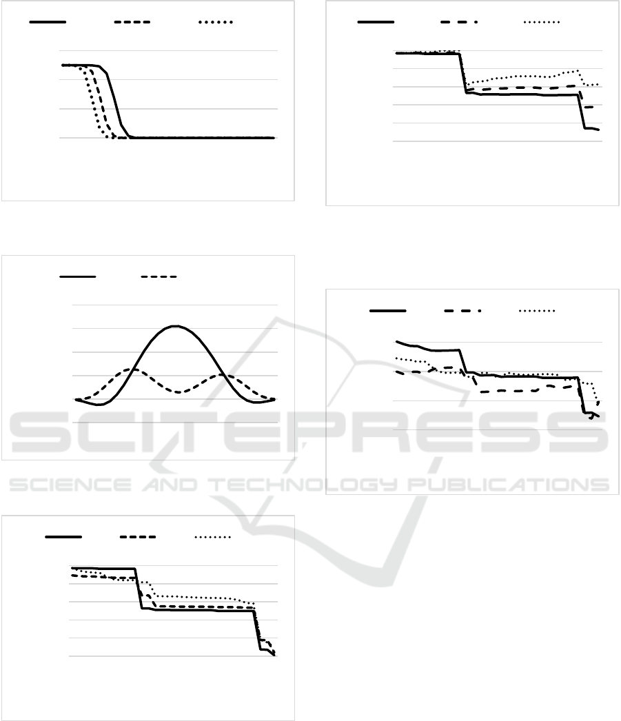
Figure 2: Plots of the eigenvalues in descending order.
.
Figure 3:Plots of the eigenvectors for the largest
eigenvalue.
. z=5.0.
Figure 4: Plots of the normalized mean square error versus
the number of eigenvectors.
computed by the Jacobi method is of orthonormal
vectors automatically. Now, we set .
Figure 2 shows the eigenvalues in descending order,
if z is 3.0, 4.0 and 5.0. They are nonnegative and real
number. Figure 3 shows the real part and imaginary
part of the eigenvectors for the largest eigenvalue at
Figure 5: Plots of the normalized mean square error versus
the number of eigenvectors. Original function is added by
noise with white Gaussian. (Ex. 1) 18.0 dB SNR;(Ex. 2)
8.4dB SNR;(Ex. 3) 4.0dB SNR.
Figure 6: Plots of the mean square error versus the number
of eigenvectors for the phase without noise.
. Because of 30 dimensional vector space,
except for this, there are 29 eigenvectors.
We consider the application of the above
eigenvectors to the problem of approximating a
function. Theoretically, we deal with a problem of
expressing an arbitrary element on a finite -
dimensional Hilbert space
with an orthonormal
basis. For any element in
, by using orthonormal
basis
, we can write
(26)
where
is an inner product (Reed et al., 1972) .
Now, we set . Let us consider the set
of
all 30-tuples
(27)
where
are complex numbers.
Now, let us consider a following test function.
(28)
0
1
2
3
1 6 11 16 21 26
Eigenvalue
Eigenvalue index
z=3.0 z=4.0 z=5.0
-0,1
0
0,1
0,2
0,3
0,4
1 6 11 16 21 26
Value of the component
Index of a component in the vector
Real Imaginary
0
0,2
0,4
0,6
0,8
1
1 6 11 16 21 26
Meansquare error
n
c=1 c=2 c=3
0
0,2
0,4
0,6
0,8
1
1 6 11 16 21 26
Mean square error
n
Ex. 1 Ex. 2 Ex. 3
0
2
4
6
1 6 11 16 21 26
Error(n)
n
c=1 c=2 c=3
Band-limited Orthogonal Functional Systems for Optical Fresnel Transform
151

where c is natural number. We evenly discretize the
test function at 30 points to reconstruct by using the
eigenvectors. Figure 4 illustrates the mean square
error versus the number of eigenvectors. The
normalized mean square error is defined by
(29)
where
is the sum in Eq. (26) up to , is the
original vector and
is the
-norm. From Fig. 4,
we can see that the error decreases with increasing
number of eigenvectors used in the expansion.
Next, let us consider another following test function.
(30)
where indicates noise and is a normally distributed
deviate with zero mean and unit variance. To measure
the effect of noise on the function, we use the signal-
to-noise ratio (SNR) (Trussel, 2008). This is usually
defined as the ratio of signal power
, to noise
power
,
(31)
and in decibels
(32)
In
, the function power is usually estimated by the
simple summation
(33)
where
is the mean of the function. Figure 5
illustrates the mean square error versus the number of
eigenvectors with noise. The SNR in example 1
(Ex.1) is 18.019354, example 2 (Ex. 2) is 8.476929
and example 3 (Ex. 3) is 4.039954. From Fig. 5, we
can see that the original test function is reconstructed
in the state that is almost perfection if SNR increases.
In general, it is difficult for the small value of SNR to
reconstruct original test function completely. Figure
6 illustrates the mean square error versus the number
of eigenvectors for the phase without noise. The mean
square error is defined by
(34)
From Fig. 6, we can see also that the error decreases
with increasing number of eigenvectors used in the
expansion for the phase.
5 CONCLUSIONS
Band-limited effects with respect to Fourier
transform have already been investigated and well
known. However, those with respect to Fresnel
transform have not been studied and revealed
sufficiently. We have investigated the band-limited
effect in Fresnel transform plane. For that, we have
sought the function that its total power in finite
Fresnel transform plane is maximized, on condition
that an input signal is zero outside the bounded
region. We have shown that this leads to the
eigenvalue problems of Fredholm integral equation of
the first kind. It is important to reveal the
mathematical properties of the integral equation for
finite Fresnel transform. Orthogonal eigenfunctions
are derived from its properties. Orthogonal functional
systems are significant tools in analysing a diffraction
image. We have also shown that the eigenfunctions
corresponding to distinct eigenvalues have dual
orthogonal property. These functional systems and its
properties show clearly the relation between
functions and their Fresnel transforms. It is difficult
in general to seek the strict solution of the integral
equation. So we desired to seek the approximate
solution in practical exact accuracy. Furthermore, we
applied it to the problem of approximating a function
and evaluated the error. We confirmed the validity of
the eigenvectors for finite Fresnel transform by
computer simulations.
In this study, there are many parameters,
especially, the band-limited areas , the wave
number and the normal distance . It is necessary to
consist of orthogonal functional systems with the
optimal parameters for finite Fresnel transform in
application of an optical system. Moreover, in
general, the matrix given by discretizing the kernel of
the integral equation is not the Hermitian matrix. If
so, it is difficult to compute accurately all eigenvalues
and eigenvectors. It is also necessary to consider other
computational methods for this. Although the kernel
function was discretizing at 30 point, it is necessary
to increase the number of sampling points. Although
we considered only one dimensional Fresnel
transform, it is necessary to derive the integral
equation for the two dimensional Fresnel transform.
These become the future problems. Theoretically, it
is important to search for a spectral representation of
finite Fresnel transform which are defined as a
bounded linear operator in Hilbert space.
REFERENCES
Aoyagi, N., 1973. Theoretical study of optical Fresnel
transformations. Dr. Thesis, Tokyo Institute of
Technology, Tokyo
Aoyagi, N., Yamaguchi, S., 1973a. Functional analytic
formulation of Fresnel diffraction. Jpn. J. Appl. Phys.
12, 336-370
Aoyagi, N., Yamaguchi, S., 1973b. Generalized Fresnel
transformations and their properties. Jpn. J. Appl. Phys.
12, 1343-1350
PHOTOPTICS 2019 - 7th International Conference on Photonics, Optics and Laser Technology
152

Jerri, A. 1977. The Shannon sampling theorem –its various
extensions and applications: a tutorial review. Proc.
IEEE, Vol. 65, No. 11, 1565-1596
Ogawa, H., 2009. What can we see behind sampling
theorems? IEICE Trans. Fundam. E92-A, 688-695
Kondo, J., 1954. Integral equation. Baifukan. Tokyo (in
Japanese)
Aoyagi, T., Ohtsubo, K., Aoyagi, N., 2018. Fredholm
integral equation for finite Fresnel transform. In 6th
International Conference on Photonics, Optics and
Laser Technology.
Slepian, D., Pollak, H., 1961. Prolate spheroidal wave
functions, Fourier analysis and uncertainty –I. Bell
Syst. Tech. J. 40, 43-63
Landau, H., Pollak, H., 1961. Prolate spheroidal wave
functions, Fourier analysis and uncertainty –II. Bell
Syst. Tech. J. 40, 65-84
Landau, H., Pollak, H., 1962. Prolate speroidal wave
functions, Fourier analysis and uncertainty-III:The
Dimension of the space of essentially time- and band-
limited signals. Bell Syst. Tech. J. 41, 1295-1336
Slepian, D., 1964. Prolate spheroidal wave functions,
Fourier analysis and uncertainty –IV. Bell Syst. Tech.
J. 43, 3009-3058
Slepian, D., 1978. Prolate spheroidal wave functions,
Fourier analysis and uncertainty –V. Bell Syst. Tech. J.
57, 1371-1430
Itoh, Y., 1970. Evaluation of aberrations using the
generalized prolate spheroidal wavafunctions. J. Opt.
Soc. Am. 60, 10-14
Anton, H., Busby, R., 2003. Contemporary linear algebra.
John Wiley & Sons, NJ
Press, W., Teukolsky, S., Vettering, W., Flannery, B., 1992.
Numerical Recipes in C. 2
nd
edition, Cambridge
University Press, Cambridge
Reed, M., Simon, B., 1972. Methods of modern
mathematical physics. Vol. 1, Academic Press, New
York
Trussel, H., Vrhel, M., 2008. Fundamentals of Digital
Imaging. Cambridge University Press, New York
Goodman, J., 2005. Introduction to Fourier optics. 3
rd
edition, Roberts & company, Colorado
APPENDIX
The delta function can be defined as follows
(Goodman, 2005);
sinc
(35)
where
sinc
sin
(36)
Noting that
exp
exp
exp
sin
(37)
we can define
as following.
sin
exp
exp
(38)
We conclude that
(39)
Band-limited Orthogonal Functional Systems for Optical Fresnel Transform
153
