Data-driven Identification of Causal Dependencies in Cyber-Physical
Production Systems
Kaja Balzereit
1
, Alexander Maier
1
, Bj
¨
orn Barig
2
, Tino Hutschenreuther
2
and Oliver Niggemann
1,3
1
Fraunhofer IOSB-INA, Fraunhofer Center for Machine Learning, Langenbruch 6, Lemgo, Germany
2
IMMS GmbH, Ehrenbergstraße 27, Ilmenau, Germany
3
Institute Industrial IT, OWL University of Applied Sciences, Lemgo, Germany
Keywords:
Machine Learning, Causal Dependencies, Cyber-Physical Production Systems, Case-based Reasoning, Timed
Automaton, Decision Tree Classifier, Principal Component Analysis, Data Science.
Abstract:
Cyber-Physical Systems (CPS) are systems that connect physical components with software components.
CPS used for production are called Cyber-Physical Production Systems (CPPS). Since the complexity of these
systems can be very high, finding the cause of an error takes a lot of effort. In this paper, a data-driven approach
to identify causal dependencies in cyber-physical production systems (CPPS) is presented. The approach is
based on two different layers of learning algorithms: one low-level layer that processes the direct machine
data and a higher-level learning layer that processes the output of the low-level layer. The low-level layer is
based on different learning modules that can process differently typed data (continuous, discrete or both). The
high-level learning algorithms are based on rule-based and case-based reasoning. Thus, causal dependencies
are detected allowing the plant operator to find the error cause quickly.
1 INTRODUCTION
In recent years, both the required product diversity
and the flexibility in production facilities have in-
creased significantly. As a result of this development,
the complexity of the production facilities used has
also increased greatly, which in the long run leads
to excessive demands on the plant operators (Sauer,
2014).
In these systems, errors can occur that lead to a
bad product quality or plant standstill. The search for
the cause of an error has always posed major chal-
lenges to plant operators. Even if error messages are
presented to the operator (e.g. over a control desk),
the connection between these messages and the cause
of the errors is not easily drawn. Since the error does
not always coincide with the message at the control
station, this shift not only leads to misleading error
messages, but also triggers subsequent errors (chain-
ing effect) that are not necessarily explained by the
original problem.
Usually the search for the cause of an error is car-
ried out manually (by the operator) during a plant
standstill. In most cases, however, the operator of
the production plant is not the plant manufacturer, as
the production facilities are often purchased. Thus,
a detailed knowledge of the plant behaviour and the
causes of possible errors is missing. For this reason,
employees must be specially trained or the relevant
experts must arrive. An automatic search for the cause
of the error is usually not possible, as this would re-
quire the causalities between the cause and the associ-
ated effect to be known. The longer a cause of failure
needs to be searched, the longer the production plant
is not working. Accordingly, the cost of a production
loss adds up to the duration of the outage. These costs
could be avoided or at least significantly reduced by
an automatic analysis of the cause of an error.
As part of Germany’s platform industry 4.0, the
topic of intelligent assistance systems is being re-
searched intensively (Federal Ministry for Economic
Affairs and Energy, 2016). This includes diagnosis,
planning, and physical assistants. In particular, di-
agnostic assistants contribute to this, but there is still
a need for research for diagnostic assistants who can
learn the causalities between an event and the corre-
sponding effect in the system. Here, it is important to
learn causality in locally limited modules, but also in
distributed systems.
In order to solve the problem, we propose a solu-
tion which addresses the topics of
592
Balzereit, K., Maier, A., Barig, B., Hutschenreuther, T. and Niggemann, O.
Data-driven Identification of Causal Dependencies in Cyber-Physical Production Systems.
DOI: 10.5220/0007362005920601
In Proceedings of the 11th International Conference on Agents and Artificial Intelligence (ICAART 2019), pages 592-601
ISBN: 978-989-758-350-6
Copyright
c
 2019 by SCITEPRESS – Science and Technology Publications, Lda. All rights reserved

1. data-driven detection of causality to help finding
the technical cause of a problem and
2. implementation of local diagnostic assistants.
The assistance system includes the learning algo-
rithms, the anomaly detection as well as the recog-
nition of causal relationships for the identification of
the causes of the error. When using machine learning
algorithms to counteract these problems, one often
meets the problem of specification: Each algorithm
is well suited for a specific problem making it hard to
find a single algorithm well suited for complex prob-
lems. The scientific question addressed in this paper
is how to efficiently combine different machine learn-
ing algorithms so even complex problems can be han-
dled well.
The contribution of this paper is as follows:
1. We present a new algorithm structure to detect
causal dependencies in a data-driven way and
present them in a human-understandable form.
The structure is based on two different layers.
One low-level learning layer that directly pro-
cesses machine data and a high-level learning
layer that connects the output of the different low-
level modules. Thus, a combination of the differ-
ent application areas of the algorithms is possi-
ble. The output of the high-level learning layer is
a human-understandable reasoning.
2. We compare different high-level learning algo-
rithms due to their suitability to draw conclusion
about causal dependencies in CPPS.
The paper is structured in four parts: First, the
state of the art is described. Following, the algo-
rithmic structure of the diagnosis assistance system is
presented. Then, a discussion of the applicability of
the algorithms concerning a specific application case
is given. Last, the topic is concluded and an outlook
to future work is given.
2 STATE OF THE ART
Generally speaking, model-based approaches use a
model to compare the system behaviour with the
model predictions while the system is running. In par-
allel, model-based approaches try to find coherences
between the symptom and the error cause (Voigt et al.,
2015; Van Harmelen et al., 2008).
For diagnosis, mostly models describing the de-
pendency between a root and its consequences are
used, for example Fault Tree Analysis (Ahmad and
Hasan, 2015; Schilling, 2015) or Event Tree Analy-
sis (Ferdous et al., 2009). Both methods are based on
Boolean algebra and probability theory.
To train these models to diagnose failures often a
lot of expert knowledge is needed (Niggemann and
Lohweg, 2015). Since this knowledge is not avail-
able in most cases, data-driven approaches are more
applicable. These approaches are based on the data
generated by the system (Fullen et al., 2017).
Other methods that can be used to learn the normal
behaviour automatically and to diagnose errors are for
example self-organizing maps (Frey, 2012), Bayesian
networks (Runkler, 2012), neural networks (Jaber and
Bicker, 2016), Support Vector Machines (Demetgul,
2013) or fuzzy logic (Wang et al., 2015).
Causality is the relation between root and symp-
tom. Based on an observed error, the goal is to find
the root of this error. However, when the causal de-
pendencies are unknown, the interpretation of obser-
vations is necessary. Statistical methods can be ap-
plied to analyse causal dependencies data-based.
One of the first approaches was developed by
Granger (Granger, 1969). This approach compares
two autoregressive models of delayed variable values.
When the regression gets better due to this delay, the
hypothesis is that the variable with the greater delay
has an impact on the other.
Another approach is presented by Horch (Horch,
2000): Based on the cross-correlation function, the
maximal absolute value of the function and the cor-
responding time delay are used for the description of
the causal dependency.
Schreiber presents a concept for the analysis of
causal dependencies that is based on transfer entropy
(Schreiber, 2000). Assuming that one variable pre-
dicts future values, the reduction of insecurity is mea-
sured.
Another possibility is given by the use of Bayesian
networks (Eaton and Murphy, 2007). They were ex-
tended to also model the dynamic behaviour of real-
world systems, which can be used to find causal de-
pendencies.
Bauer proposes various algorithms based on
nearest-neighbour methods (Bauer, 2005). The value
of a certain variable is predicted by the value of a dif-
ferent variable.
Our approach differs from past research since it
is based on a two-level learning algorithm. The low-
level learning is based on established algorithms for
the detection of coherences in machine data like neu-
ral networks (Jaber and Bicker, 2016) and Support
Vector Machines (Demetgul, 2013). Additionally,
Timed Automata as presented by Maier (Maier, 2014)
and a combination of a Principal Component Analy-
sis (PCA) combined with a Nearest Neighbour search
(Eickmeyer et al., 2015) are used. This basis is com-
pleted by a high-level learning layer, that combines
Data-driven Identification of Causal Dependencies in Cyber-Physical Production Systems
593

the output of the different low-level modules to draw
causal conclusions. Thus, the different application ar-
eas of the different algorithms are combined. This
makes it possible to handle differently shaped data
(periodic, static, continuous, discrete, ...).
3 CAUSALITY ANALYSIS
ALGORITHM
The basis for a successful diagnosis in a production
plant is the exact knowledge of each individual state.
There are a lot of machine learning methods that
model plant behaviour. Each of these methods are in-
tended for a specific field of application (e.g. timing
machines for the timing of discrete events, or Princi-
pal Component Analysis (PCA) for the analysis of a
set of continuous signals). In addition, due to com-
binatorics, it is not possible to learn a single model
for a distributed system, since the presence of parallel
processes can increase the complexity of the model
enormously (Maier et al., 2011). The aim of this ap-
proach is a high-level learning layer, (see Figure 1),
which is able to infer causal dependencies out of the
outputs of different local models.
3.1 General Structure
The purpose of assistance systems is to support the
employee in various tasks, such as the fault diagno-
sis as well as the reduction of the system complexity.
Many machine learning methods are unsuitable for
the direct use in diagnosis assistance systems because
the output cannot be interpreted in an intuitive manner
by humans. For example, when using neural networks
it is not easy to comprehend how the neural network
calculated its output. Since the input is propagated
by a lot of hidden layers, a direct coherence cannot be
drawn. However, this is a prerequisite for the success-
ful deployment of a diagnosis assistance system. The
problem here is that machine learning typically works
on a low-level (sub-symbolic level). In order to make
the results accessible to humans, however, algorithms
must be developed that work on a high-level (sym-
bolic level).
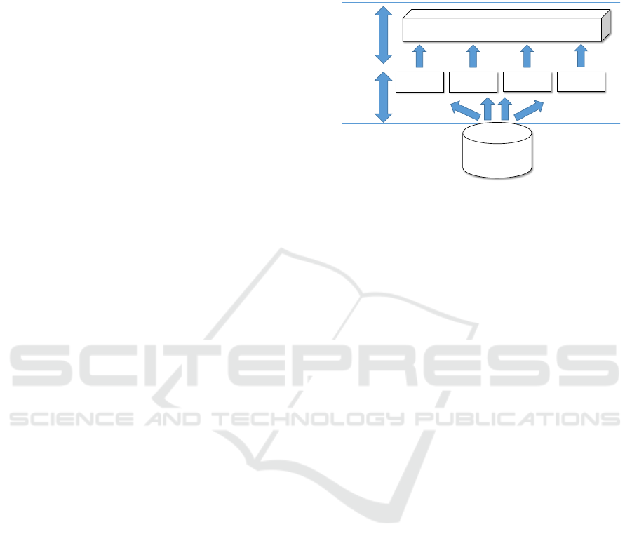
Figure 1 illustrates the structure of the assistance
system presented in this approach. The machine
data first is given to a number of low-level mod-
ules. These modules are represented by different al-
gorithms that have different advantages and disadvan-
tages. Here, only models limited to machine compo-
nents are learned. These can cover certain aspects of
behaviour (discrete, continuous, ...). The high-level
earning methods are designed to combine all the un-
derlying techniques. The data is prepared in a human-
understandable form, e.g. by integration of seman-
tic knowledge (naming the system states) or an inter-
pretable structure (e.g. ”if ... then” - rules).
Machine data
000101010100110
101010101000011
101011100100011
Learning based on multiple sources (e.g. rule-learning)
High-level
learning
Low-level
learning
Module 1
Module 2
Module 3
Module 4
Figure 1: Algorithmic structure of the global diagnosis as-
sistant.
3.2 Low-level Learning
Every module in the low-level is represented by a ma-
chine learning algorithm. Thus, for each module one
model is trained that is used to give information about
the current status of the machine. Each algorithm is
specialized on different properties: Some algorithms
are able to process continuous data, others work on
discrete data. In the presented approach, the machine
data is separated based on its type so each algorithm
gets that data it can process best.
Many algorithms used for anomaly detection need
to be trained with the help of a labelled dataset be-
fore they can be used. We call these algorithms offline
since the model is learned once before the prediction
can be done. Algorithms that adapt their model dur-
ing the prediction are called online. These algorithms
do not need to be trained before they are used but im-
prove the model during the prediction.
In the following, different algorithms used for
the detection of causal coherences in CPPS are pre-
sented. An online algorithm based on Timed Au-
tomata can process discrete data. An offline work-
ing combination of a Principal Component Analysis
and a Nearest-Neighbour Classification is used to find
patterns in continuous data. To detect outliers in the
machine data, an online working algorithm is used.
Online Timed Automaton Learning Algorithm.
Timed Automata are often used for programming pro-
duction systems and are therefore suited for modeling
a technical process.
A Timed Automaton is a tuple A =
(S, s
0
, F, Σ, T, ∆, c), where
ICAART 2019 - 11th International Conference on Agents and Artificial Intelligence
594

• S is a finite set of states, s
0
∈ S is the initial state,
and F ⊆ S is a set of final states,
• Σ is the alphabet comprising all relevant events,
• T ⊆ S ×Σ ×S gives the set of transitions. E.g. for
a transition hs, a, s
0
i, s, s
0
∈ S are the source and
destination states and a ∈ Σ is the trigger event.
• A set of transition timing constraints ∆ with δ :
T → I, δ ∈ ∆, where I is the set of time intervals.
• A single clock c is used to record the time evolu-
tion. At each transition, the clock is reset. This al-
lows only for the modelling of relative time steps.
In (Niggemann et al., 2012) and (Verwer, 2010),
the authors present an offline algorithm to identify
Timed Automata from data. Both approaches are
based on the state merging paradigm, both defining
individual state compatibility criteria. Another ap-
proach can be found in (Maier, 2014), where the
method presented identifies Timed Automata in an
online manner (Online Time Automaton Learning Al-
gorithm). For this, a different state compatibility cri-
terion is defined which is based on the values of the
signal vector.
Usually, Timed Automata are used to describe a
discrete behaviour. For the modelling of continu-
ous or hybrid behaviour, further methods like a PCA-
based anomaly detection (see next paragraph) are
needed.
In the following, the algorithm is referred to as
OTALA.
PCA-based Anomaly Detection. Eickmeyer et al.
presented an approach for anomaly detection that is
based on a Principal Component Analysis (Eickmeyer
et al., 2015). First, the input data and the training
set are transformed to a lower-dimensional euclidean
room with the use of the PCA. Then, the nearest
neighbour to the input data point is searched for in
the transformed training set. With the help of a Marr
wavelet function a probability is calculated, that de-
termines how likely the given point is part of the nor-
mal space.
This algorithm works on continuous data that sat-
isfies the assumption that most of the information is
located in the direction of the maximal variance.
Many algorithms used for the determination of an
observation being part of the normal space is done us-
ing fixed thresholds. These thresholds are given using
expert knowledge. A great advantage of the presented
approach is that it needs less expert knowledge: Since
a Marr wavelet function that uses probabilities is used,
no fixed threshold is needed. The expert knowledge
is only needed when generating the training set since
in the training set only normal behaviour must be rep-
resented.
In the following, the algorithm is referred to as
PCNA.
Online Outlier Detection. In this paragraph, an al-
gorithm for outlier detection is presented. In general,
it is not useful to apply this method to discrete data,
therefore, in the presented approach it is only used to
process continuous data. The algorithm works com-
pletely online and does not need to be trained before
its use. Only the mean value and the standard devia-
tion are needed for this algorithm. In the following,
formulas to calculate these online are presented.
Based on these values, the data is checked and la-
belled okay or faulty. Therefore, first the mean value
for the n −th data point E
n
is calculated recursively
for every component j by
E
n
j
=
n −1
n
E
n−1
j
+
1
n
x
n
j
∀j ∈{1, 2, ..., M}, (1)
where E
n−1
j
describes the mean value for the n −1
st
data point of component j and x
n
j
describes the current
observation. Note that E
1
j
= x
1
j
and dim(x
n
) = M.
Similar, the variance can be calculated recursively
by
V
n
j
=
1
n

(n −1) ·V
n−1
j
+
n −1
n
(E
n−1
j
−x
n
j
)
2

(2)
∀j ∈{1, 2, ..., M} and V
1
= 0. Based on this, the cur-
rent standard deviation can be calculated by
σ
n
=
√
V
n
. (3)
With this information an outlier detection can be done
by checking if a given data point x
n
fulfils the equation
|x
n
j
−E
n
j
| < r ·σ
n
j
∀j ∈{1, 2, ..., M} (4)
with a r ∈ R. r has to be defined by an expert since it
is a measurement how far data points may differ from
previous data points. If equation (4) is satisfied for
every component of x
n
, it is labelled okay, otherwise
it is labelled as an outlier.
Other Algorithms. The algorithmic structure (see
figure 1) offers a lot of flexibility concerning the low-
level modules, therefore many different algorithms
may be used. Since self-organizing maps (Frey,
2012), Bayesian networks (Runkler, 2012), neural
networks (Jaber and Bicker, 2016), Support Vector
Machines (Demetgul, 2013) and fuzzy logic (Wang
et al., 2015) have been used for the data-driven diag-
nosis in real-world applications, their suitability as a
low-level module is high. Additionally, established
implementations of these algorithms exist, so that the
integration effort is low.
Data-driven Identification of Causal Dependencies in Cyber-Physical Production Systems
595

3.3 High-level Learning
High-level learning enables the combination of dif-
ferent model formalisms (from low-level-learning) as
well as the combination of models from different
modules, which in turn allows a global system mod-
elling.
3.3.1 Rule-based Reasoning
In particular, rule-based learning methods are promis-
ing at this point because they can determine causal
relationships due to their ”if ... then ...” - struc-
ture. Based on different learning methods of low-level
learning, the individual modules are able to broad-
cast messages about the condition. The goal now is
to evaluate these ”broadcast messages” for existing
causalities. Figure 2 shows a minimal example of how
learning high-level rules can be used to combine low-
level models to deduce causal relationships. A similar
rule might look like this:
If conveyor A is standing, then module B will
not get a bottle.
The technical background of this rule would be the
following:
If module A is in state 4 and t > 5s, then mod-
ule B is in error state F.
The learned automaton provides further details on the
individual states: State 4 of module A corresponds
to ”conveyor belt”, while state F of module B cor-
responds to the error state ”bottle is missing”. The
underlying state machines can be learned using algo-
rithms like (Hy-)BUTLA (Niggemann et al., 2013).
Here, an approach based on different decision tree
methods is used to generate the decision rules. First,
generating rules with the use of a single decision tree
then the use of random-forest classifiers is presented.
2
1
4
3
1
3
2
F
Module A
Module B
Figure 2: Rule-learning to detect causal dependencies be-
tween error cause and anomaly.
Decision Tree Learning. One way to realize rule-
based learning is by the usage of decision tree al-
gorithms. A great advantage of decision trees is
the high interpretability and transparency (Murphy,
2012). Decisions made with the help of decision trees
are easy to understand, since every node represents a
single decision rule. When applying a rule the output
leads to further nodes with further decision rules. An
”if ... then ...” - structure is found easily.
Trees can process continuous as well as discrete
input data (Murphy, 2012). Continuous data can be
separated using inequations, discrete data can be enu-
merated. So, the different output of the low-level
modules (like a discrete state from (Hy-)BUTLA or
a continuous probability from the PCNA) can both be
interpreted and processed.
When handling trees often the problem of overfit-
ting is occurring. Trees are very unstable and strongly
depending on the training data (Murphy, 2012). Thus,
when different changes are applied to the training
data, the shape of the decision tree may vary largely.
For the application case of anomaly detection in
CPPS, this means that the training data should ap-
proximately consist of so many data points describing
correct machine behaviour as data points describing
anomalies.
There are many different methods to find the opti-
mal partition of a dataset (Murphy, 2012). The most
popular methods are CART (Breiman et al., 1984),
ID3 (Quinlan, 1986) and C4.5 (Quinlan, 1993). Here,
the implementation of scikit-learn is used which is
based on the CART algorithm (Pedregosa et al.,
2011).
Random-forest Classifier. Since using a single tree
as classifier can lead to a high variance in the result,
decision tree methods are expanded to methods han-
dling more than a single tree. These methods are
called Forest Classification methods.
Therefore N ∈ N differently shaped decision trees
are trained. The different shape of the decision trees
are achieved by using different training sets. They are
randomly chosen from the original training set.
The prediction f (x) of the forest for an input vec-
tor x is then calculated by
f (x) =
1
N
N
∑
n=1
f
n
(x) (5)
where f
n
(x) represents the prediction of the n-th tree.
The result calculated by forest classifiers cannot
be interpreted directly. Since it is a weighted average
of outputs by a set of trees, the interpretation is more
complex than the interpretation of the output of a sin-
gle tree. This makes it more difficult to extract the
causal dependencies searched.
3.3.2 Case-based Reasoning
As an alternative to rule learning, case-based reason-
ing (CBR) (including pattern recognition and clus-
ICAART 2019 - 11th International Conference on Agents and Artificial Intelligence
596

tering algorithms) can be used to detect causal de-
pendencies. CBR methods are based on reasoners,
that remember previous situations similar to the cur-
rent one and propose a solution approach (Kolodner,
1993).
When using CBR methods, one challenge is how
to generate the case base. Previous cases need to be
indexed and stored in a case memory (Xu, 1994). An-
other challenge is how to define similarity between
cases (Fullen et al., 2017).
To apply CBR to a data set, the data is searched
for frequently recurring patterns, which can be used
to detect relationships that may be useful for further
analysis, e.g.
Every morning, energy consumption increases
dramatically.
or
State pairs [Module A / State 4] and [Module
B / State F] often appear together.
The second-mentioned pattern corresponds to the
rule from the previous section. However, caution
is advised not to confuse observed correlations with
causality.
For each detected error, a case is stored in the case
base. Subsequently, similarity measures are learned
which are functions of the low-level output describ-
ing a cause. For new cases, similar cases are searched
using the similarity measures. It is important that the
cases are formalized with features. Furthermore, re-
lationships between these anomalies and causes of er-
rors are stored in a database and thus provide a mem-
ory for the diagnostic assistant, which can be used in
future diagnoses to identify anomalies even more re-
liably and assign them to a cause.
The core of every CBR strategy is the case base.
It consists of cases that occurred in the past. It is im-
portant that the cases are well suited for the prediction
about new cases (Kolodner, 1993).
For the high-level learning, the case base consists
of output generated by the low-level modules. There-
fore, the machine data is propagated by the low-level
modules. The output represents one case. Since the
output of the low-level modules can be both, contin-
uous (e.g. a probability from the PCNA) and discrete
(e.g. a machine status by OTALA or a cluster number
by a clustering method), the case is represented by a
hybrid data vector. Then the case is labelled with the
error cause by the machine operator.
So, a case is described by a vector y and an
error cause, coded by an integer g ∈ N. The
case base then can be described as a set of tuples
Y = {(y
1
, g
1
), (y
2
, g
2
), ...}.
When using CBR strategies a major challenge is
the determination of similarity of data points (Fullen
et al., 2017). Since the high-level learning algorithm
has to handle hybrid data, a similarity measure that
can handle both, continuous and discrete values, is
needed. In the following, a hybrid approach based
on the euclidean distance and the discrete metric is
presented.
Let x = (c
1
, d
1
) be the current (unlabelled) out-
put of a machine data set propagated by the low-level
modules where c
1
∈ R
k
stores the continuous val-
ues and d
1
∈ R
l
stores the discrete values. For this
data point, the most similar case in the case base Y is
searched. Therefore, a definition of similarity has to
be given.
Let (y, g) be a tuple from the case base Y which
similarity to x shall be determined. y can be de-
scribed by y = (c
2
, d
2
) with c
2
∈R
k
representing the
continuous values and d
2
∈ R
l
representing the dis-
crete values.
For the similarity measure of the continuous val-
ues, first, the data is scaled using the current mean
value and the current standard deviation. Let E
c
be
the current mean value of the continuous data (recur-
sively calculated using (1)) and σ
c
be the current stan-
dard deviation of the continuous values (recursively
calculated using (2)). Then, every component of c
1
can be scaled by
˜c
1
i
=
c
1
i
−E
c
i
σ
c
i
∀i ∈ {1, ..., k} (6)
(analogue for ˜c
2
). Based on this, the continuous dis-
tance d
c
of x and y is defined using the euclidean
distance
d
c
(x, y) :=
k
˜c
1
− ˜c
2
k
2
=
v
u
u
t
k
∑
i=1
( ˜c
1
i
− ˜c
2
i
)
2
. (7)
Calculating the similarity of the discrete values can-
not be done as simple as the similarity for the con-
tinuous values since discrete values in general are not
interval typed, i.e. if a module is stuck in state 4 this
is not twice as bad as if the module is stuck in state
2. Therefore, a measurement just scoring if there is a
difference between two states is needed. This can be
done by using the discrete metric
δ(a, b) :=
(
1 if a 6= b
0 if a = b.
(8)
For the definition of the discrete distance d
d
of x and
y the discrete metric δ is extended to
d
d
(x, y) :=
l
∑
i=1
δ(d
1
i
, d
2
i
). (9)
Data-driven Identification of Causal Dependencies in Cyber-Physical Production Systems
597

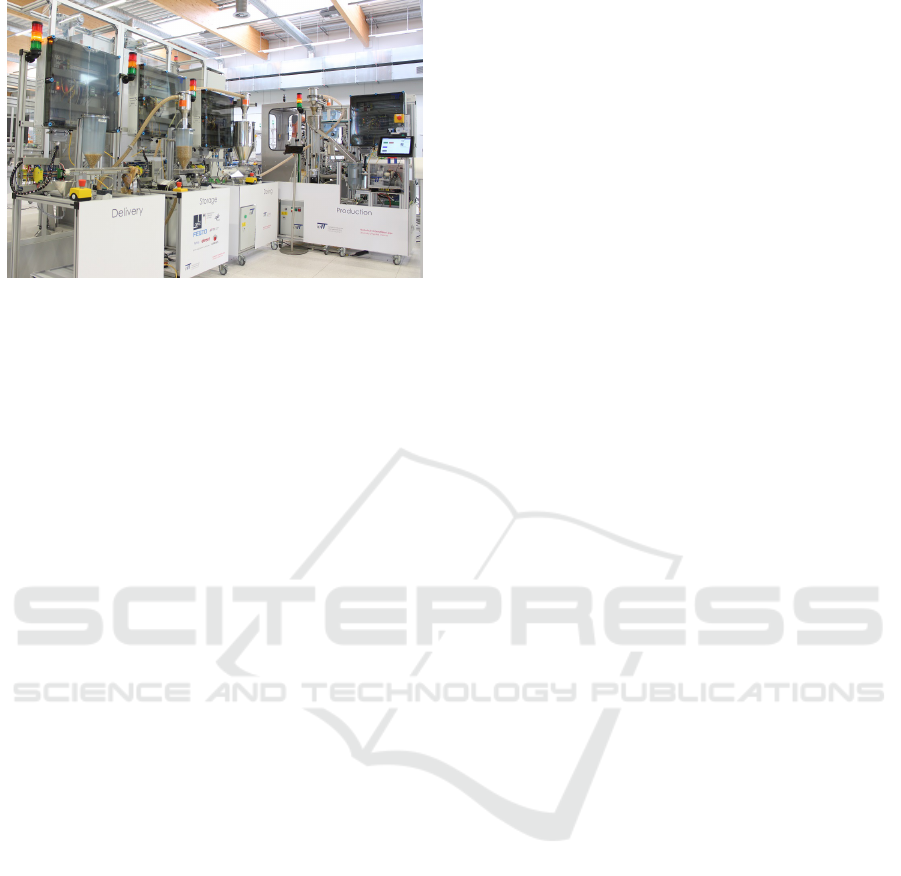
Figure 3: Graphical image of the Versatile Production Sys-
tem of the SmartFactoryOWL. The VPS consists of four
different modules (Delivery, Storage, Dosing and Produc-
tion).
Thus, for two given data points x and y a discrete as
well as a continuous distance can be calculated. To
determine the most similar case in the case base Y ,
a priority between these two measurements has to be
defined.
The most similar data point y
x
∈Y = {y
1
, y
2
, ...}
then is defined by
y
x
= arg min
y∈D
y
{d
c
(x, y)} (10)
with
D
y
= arg min
y∈Y
{d
d
(x, y)}. (11)
This means, that first the data points in Y are searched,
which discrete distance is smallest (note that this can
be more than one data point). These are represented
by the set D
y
. From these data points, that one is
searched, which continuous distance to the given data
point x is smallest. That data point is the most similar
case y
x
.
4 DISCUSSION
In this section, a discussion of the different proposed
methods based on an industrial use case is given.
4.1 Description of the Industrial Use
Case
For the discussion of the presented solution approach
a demonstrator of the SmartFactoryOWL is used. It is
a versatile production system which represents typical
industry processes (see figure 3).
The system consists of four different modules.
The first is a delivery module where material is in-
put. From that module, the material is transported to
the second module which task is to store and trans-
port material. After that module a dosing module is
placed, which fills the material into bottles. Finally,
the material is transported to the production module
where it is transported through a blow pipe into a
heater. The system produces more than 200 signals
(Bunte et al., 2016).
These signals are continuous or discrete (boolean
or integer). As described above, they are separated so
that each low-level module gets the data that the algo-
rithm is best suited for. E.g. the Principal Component
Analysis as well as clustering methods get continu-
ous values while the Timed Automata (OTALA) can
handle discrete data.
4.2 Application of Presented Methods
The presented high-level learning methods are com-
pared regarding their interpretability, the implemen-
tation effort and their suitability for the presented use
case.
Training. To apply these methods, first, a training
set has to be generated. It needs to contain correct as
well as false behaviour of the machine.
Therefore, the machine is run and the machine
data is propagated by the low-level modules. The
different low-level algorithms calculate predictions
based on their individual training. After that, the out-
puts of the low-level modules are collected and stored.
When no error occurred, the data points are labelled
with an error code representing OK. After that, typ-
ical errors (missing bottle, blockage, ...) are inserted
into the system. The related datasets are labelled with
the specific integer coding the error and its cause. By
doing so, a dataset containing the output of low-level
data and the related machine behaviour (error and its
cause) is created.
Single Decision Tree Classifier. With this dataset
the training of the different high-level modules is
done. When training a decision tree using the CART
algorithm, the whole training set is used. It is impor-
tant to prevent the tree from overfitting by defining a
maximum depth and a minimum split.
Figure 4 shows an example of a decision tree
learned with the CART algorithm. The CART al-
gorithm is based on a greedy search to separate the
differently labelled data points in the given training
set. With this greedy search, the result of the PCNA
r
PCNA
is the most expressive value to separate the
given training set. When a condition is satisfied, the
left branch is used for further separation. In contrast,
when a condition is not satisfied, the right branch is
ICAART 2019 - 11th International Conference on Agents and Artificial Intelligence
598

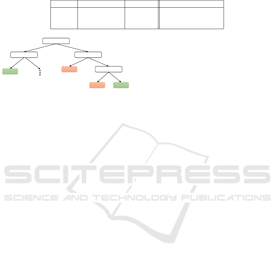
Table 1: Comparison of single decision tree classifiers (SDTC), random forest classifiers (RFC) and case-based reasoning
(CBR) is given using the attributes interpretability, implementation effort and suitability.
method interpretability suitability implementation effort
SDTC high medium low
RFC low low low
CBR high high high
𝑟
𝑃𝐶𝑁𝐴
≤ 0.05
𝑟
𝑂𝑇𝐴𝐿𝐴
= 1 𝑟
𝑁𝑒𝑢𝑁𝑒𝑡
= 1
Error
OK
𝑟
𝑂𝑇𝐴𝐿𝐴
= 2
Error OK
Figure 4: Decision Tree learned with the CART Algorithm
and the machining data from the VPS.
used. In the example, if the condition r
PCNA
≤ 0.05
is satisfied, the result of OTALA r
OTALA
is checked.
Practically, this means the machine is checked for its
current status. Based on this status, a decision is made
whether an error has occurred or not or if further low
level modules have to be checked.
Based on this decision tree, decision rules like
When r
PCNA
≤ 0.05 and r
OTALA
= 1 then OK.
can be derived. Practically speaking, this means
When the PCNA module labels the data points
okay and the machine is in state 1, no error
has occurred.
Since this rule is easy to understand by a human op-
erator, the interpretability of the Decision Tree Clas-
sifier is high.
Random Forest Classifier. When using Random
Forest Classifiers, multiple (for example ten) deci-
sion trees are created using different training data sets.
These sets are randomly created from the initial train-
ing data set. The trees created this way differ in their
structure and therefore even may differ in their pre-
dictions. For example, when using ten decision trees
for an online prediction while the machine is running,
eight may predict OK and two may predict ERROR.
For a classification of a single data point, a number
of classification rules is used. This makes the predic-
tion hard to interpret since the rules even may contra-
dict each other. Thus, a unique reasoning for the error
cause is impossible.
Case-based Reasoning. Using the training data set
described above, the case base for the CBR strategy
can be created. Defining the case base as the whole
training data set would make the search for the most
similar case of a given data point last very long. Thus,
a representative subset of the case base is selected.
Cases representing normal and false behaviour are
chosen.
For example, a case in the case base can be
r
OTALA
= 1, r
PCNA
= 0.025, r
NeuNet
= 1, (12)
labelled with OK. This case is representing correct
behaviour. Another case could be
r
OTALA
= 2, r
PCNA
= 0.95, r
NeuNet
= 0, (13)
labelled with a specific code describing the error and
its cause.
When running the machine, the machine data is
first propagated by the low-level modules. So, a data
point, for example
r
OTALA
= 2, r
PCNA
= 0.85, r
NeuNet
= 0, (14)
is generated. This data point is compared to the
known cases using the similarity measurement pre-
sented above. The most similar case - here
r
OTALA
= 2, r
PCNA
= 0.95, r
NeuNet
= 0 (15)
- is chosen and its error cause and a solution approach
are presented to the machine operator. The machine
operator then can check for the proposed error and
correct it. If the error cause is as assumed, the ma-
chine operator labels the solution approach as useful.
The current case is then added to the case base with
the related error cause and its solution.
If the solution proposal was not helpful but wrong,
the machine operator can re-label the dataset using a
proposal of possible error codes. So, the case is added
to the case base with a new solution proposal. When,
in future, a similar case occurs it is more probable
that the correct solution approach is presented since
the similarity to the currently added case probably is
the highest.
Comparison. In table 1, the three different high-
level learning methods are compared concerning their
interpretability, the implementation effort and the
suitability for the application in an industrial use case.
As mentioned above, a great advantage of single
decision trees is their high interpretability since de-
cision rules can easily be drawn from the decision
Data-driven Identification of Causal Dependencies in Cyber-Physical Production Systems
599

tree. Established algorithms like CART can be used,
so the implementation effort is rated low. Since over-
fitting to the given training set is a big problem of
single trees, the suitability for the application is rated
medium.
Since the prediction is based on multiple decision
trees, the interpretation of the result of a random for-
est classification is difficult. Contradicting decision
rules may be used for the current prediction, causali-
ties cannot be found easily. For the application case,
this leads to a low rated suitability. Established algo-
rithms can be used for the implementation, the effort
for this is rated low.
Using a case-based reasoning strategy for the
learning returns a similar case from the past and the
then detected error cause. The result is easy to inter-
pret for the machine operator and the machine opera-
tor can check if the past case has occurred again. For
the implementation of a case-based reasoning strat-
egy a lot of implementation effort is needed: The
case base, consisting of representative cases, has to
be generated. Additionally, a similarity measurement
has to be defined, which is well suited for the differ-
ently typed outputs. When a case has been handled,
the case base needs to be updated. Since a relation
between past behaviour of the production machine
and current behaviour is drawn, the suitability is rated
high.
5 CONCLUSION
In this paper, a data-driven approach to identify causal
dependencies in CPPS is presented. The structure of
the presented analysis tool is based on two layers: one
low-level learning layer that directly processes ma-
chine data and a high-level learning layer that pro-
cesses the output of the low-level modules.
The low-level modules are based on established
machine learning algorithms like cluster analysis,
Timed Automata or Principal Component Analysis.
The specific algorithms are given that data, that they
are best suited for. For example, cluster analysis
works good on continuous data while Timed Au-
tomata are used to process discrete data.
The high-level learning algorithms differ in rule-
based and case-based algorithms. As rule-based algo-
rithms, decision tree classifiers based on a single tree
and on multiple trees (also named forest classifiers)
were used. Additionally, the usage of a case-based
reasoning strategy is presented. These methods are
compared concerning their interpretability, their im-
plementation effort and their suitability for the appli-
cation case. Even though the implementation effort
for a case-based reasoning strategy is high, it outper-
forms the rule-based strategies.
In future work, different algorithms for the low-
level modules will be evaluated. Since the presented
concept is very flexible, the applicability of different
algorithms can be compared quickly.
Additionally, the case-based reasoning strategy
will be improved. Since the generation of the case
base requires a lot of effort, methods to automatically
generate this are examined. Furthermore, different
similarity measurements than the presented one are
examined concerning their applicability for the spe-
cific use case of high-level learning.
ACKNOWLEDGEMENTS
This work was partially funded by the BMWi (Ger-
man Federal Ministry of Economics and Technology),
funding code IGF 19341 BG, as a part of the project
”AgAVE: Assistenzsysteme zur
¨
Uberwachug von ver-
netzten Anlagen - Herausforderungen beim Vernetzen
sowie beim Erkennen von kausalen Zusammenhngen
in Industrie 4.0 Umgebungen” (2017-2019) and par-
tially funded by the Fraunhofer Cluster of Excellence
”Cognitive Internet Technologies”.
REFERENCES
Ahmad, W. and Hasan, O. (2015). Towards formal fault
tree analysis using theorem proving. In Conferences
on Intelligent Computer Mathematics, pages 39–54.
Springer.
Bauer, M. (2005). Data-driven methods for process analy-
sis. PhD thesis, University of London.
Breiman, L., Friedman, J., Stone, C., and Olshen, R. (1984).
Classification and Regression Trees. The Wadsworth
and Brooks-Cole statistics-probability series. Taylor
& Francis.
Bunte, A., Diedrich, A., and Niggemann, O. (2016). Se-
mantics enable standardized user interfaces for diag-
nosis in modular production systems. In International
Workshop on the Principles of Diagnosis (DX), Den-
ver, CO, USA.
Demetgul, M. (2013). Fault diagnosis on production sys-
tems with support vector machine and decision trees
algorithms. The International Journal of Advanced
Manufacturing Technology, 67(9-12):2183–2194.
Eaton, D. and Murphy, K. (2007). Belief net structure learn-
ing from uncertain interventions. Journal of Machine
Learning Research, 1:1–48.
Eickmeyer, J., Li, P., Givehchi, O., Pethig, F., and Nigge-
mann, O. (2015). Data driven modeling for system-
level condition monitoring on wind power plants. In
DX@ Safeprocess, pages 43–50.
ICAART 2019 - 11th International Conference on Agents and Artificial Intelligence
600

Federal Ministry for Economic Affairs and Energy,
editor (2016). Ergebnispapier - Aspekte der
Forschungsroadmap in den Anwendungsszenarien.
Berlin.
Ferdous, R., Khan, F., Sadiq, R., Amyotte, P., and Veitch,
B. (2009). Handling data uncertainties in event tree
analysis. Process safety and environmental protection,
87(5):283–292.
Frey, C. W. (2012). Monitoring of complex industrial
processes based on self-organizing maps and water-
shed transformations. In Industrial Technology (ICIT),
2012 IEEE International Conference on, pages 1041–
1046. IEEE.
Fullen, M., Sch
¨
uller, P., and Niggemann, O. (2017). Defin-
ing and validating similarity measures for industrial
alarm flood analysis. In Industrial Informatics (IN-
DIN), 2017 IEEE 15th International Conference on,
pages 781–786. IEEE.
Granger, C. W. (1969). Investigating causal relations
by econometric models and cross-spectral methods.
Econometrica: Journal of the Econometric Society,
pages 424–438.
Horch, A. (2000). Condition monitoring of control loops.
PhD thesis, Signaler, sensorer och system.
Jaber, A. A. and Bicker, R. (2016). Industrial robot back-
lash fault diagnosis based on discrete wavelet trans-
form and artificial neural network. American Journal
of Mechanical Engineering, 4(1):21–31.
Kolodner, J. (1993). Case-based Reasoning. Artificial in-
telligence. Morgan Kaufmann Publishers.
Maier, A. (2014). Online passive learning of timed au-
tomata for cyber-physical production systems. In The
12th IEEE International Conference on Industrial In-
formatics (INDIN 2014). Porto Alegre, Brazil.
Maier, A., Vodencarevic, A., Niggemann, O., Just, R., and
Jaeger, M. (2011). Anomaly detection in produc-
tion plants using timed automata. In 8th Interna-
tional Conference on Informatics in Control, Automa-
tion and Robotics (ICINCO), pages 363–369.
Murphy, K. P. (2012). Machine Learning. A Probabilistic
Perspective. Massachusetts Institute of Technology.
Niggemann, O. and Lohweg, V. (2015). On the diagno-
sis of cyber-physical production systems: state-of-
the-art and research agenda. In Proceedings of the
Twenty-Ninth AAAI Conference on Artificial Intelli-
gence, pages 4119–4126. AAAI Press.
Niggemann, O., Stein, B., Voden
ˇ
carevi
´
c, A., Maier, A., and
Kleine Buning, H. (2012). Learning behavior models
for hybrid timed systems. In Twenty-Sixth Conference
on Artificial Intelligence (AAAI-12).
Niggemann, O., Vodencarevic, A., Maier, A., Windmann,
S., and B
¨
uning, H. K. (2013). A learning anomaly de-
tection algorithm for hybrid manufacturing systems.
In The 24th International Workshop on Principles of
Diagnosis (DX-2013), Jerusalem, Israel.
Pedregosa, F., Varoquaux, G., Gramfort, A., Michel, V.,
Thirion, B., Grisel, O., Blondel, M., Prettenhofer,
P., Weiss, R., Dubourg, V., Vanderplas, J., Passos,
A., Cournapeau, D., Brucher, M., Perrot, M., and
Duchesnay, E. (2011). Scikit-learn: Machine learning
in Python. Journal of Machine Learning Research,
12:2825–2830.
Quinlan, J. R. (1986). Induction of decision trees. Machine
learning, 1(1):81–106.
Quinlan, J. R. (1993). C4.5: Programs for Machine Learn-
ing. Morgan Kaufmann Publishers Inc., San Fran-
cisco, CA, USA.
Runkler, T. A. (2012). Data Analytics. Springer.
Sauer, O. (2014). Information technology for the factory of
the future–state of the art and need for action. Proce-
dia CIRP, 25:293–296.
Schilling, S. J. (2015). Contribution to temporal fault tree
analysis without modularization and transformation
into the state space. arXiv preprint arXiv:1505.04511.
Schreiber, T. (2000). Measuring information transfer. Phys-
ical review letters, 85(2):461.
Van Harmelen, F., Lifschitz, V., and Porter, B. (2008).
Handbook of knowledge representation, volume 1. El-
sevier.
Verwer, S. (2010). Efficient Identification of Timed Au-
tomata: Theory and Practice. PhD thesis, Delft Uni-
versity of Technology.
Voigt, T., Flad, S., and Struss, P. (2015). Model-based fault
localization in bottling plants. Advanced Engineering
Informatics, 29(1):101–114.
Wang, T., Zhang, G., Zhao, J., He, Z., Wang, J., and P
´
erez-
Jim
´
enez, M. J. (2015). Fault diagnosis of electric
power systems based on fuzzy reasoning spiking neu-
ral p systems. IEEE Transactions on Power Systems,
30(3):1182–1194.
Xu, L. D. (1994). Case based reasoning. IEEE potentials,
13(5):10–13.
Data-driven Identification of Causal Dependencies in Cyber-Physical Production Systems
601