Operations for Shape Transformations based on Angles
Momo Tosue, Sosuke Moriguchi and Kazuko Takahashi
Kwansei Gakuin University, 2-1 Gakuen, Sanda, Hyogo, Japan
Keywords:
Symbolic Expression, Diagram, Abstract Rewriting System, Qualitative Spatial Representation.
Abstract:
We propose a symbolic expression for a qualitative shape of an object in the sequence of rotation angles of
edges. We give a drawing algorithm for the expression based on rewriting strings and prove that we can draw
a figure on a two-dimensional plane, for a consistent expression. We also refine this algorithm as an abstract
rewriting system to represent shapes of figures and their changes, and prove that the system has confluence
and termination.
1 INTRODUCTION
Work in the field of artificial intelligence involves
symbolic treatment of spatial data. When we look
at images or diagrams, it is easier to recognize the
features thereof (shape, relative position, and relative
size). However, when we discuss the properties of
such features, it is appropriate to express the figure
symbolically. Symbolic treatment creates a represen-
tation amenable to human understanding and enables
the use of computational tools in the formalization,
whereas numerical data cannot be treated in this man-
ner.
Qualitative Spatial Temporal Reasoning is the
subfield of knowledge representation and symbolic
reasoning (Ligozat, 2011). It focuses on certain as-
pects of an object, and reasons by reference to those
aspects, without using precise numerical data. Ap-
plication areas including robot navigation and ge-
ographic information systems have been proposed.
Both shapes and their transformations are considered
as important aspects in these applications, and sev-
eral studies have explored the symbolic representation
of object shapes in the two-dimensional plane. Most
represented object shapes by tracing the boundaries
(Leyton, 1988; Galton and Meathrel, 1999; Museros
and Escrig, 2004; Schlieder, 1996; Kulik and Egen-
hofer, 2003; Gottfried, 2003; Gottfried, 2004). A
boundary is a closed figure usually divided into seg-
ments. The boundary is thus represented as a se-
quence of segments, sometimes combined with rela-
tionships between adjacent segments. The shape fea-
tures distinguish straight from curved lines, the sizes
of edges and angles. Cohn took a different approach
in which an outline is not traced to represent a qualita-
tive shape of an object (Cohn, 1995). He developed a
representation using relationships over regions. Con-
vexity was considered, with a hierarchical focus on
the difference between the region occupied by a given
object and its convex hull. Tosue et al. developed a
symbolic expression incorporating concavity, tangent
points, and divisions of an object, as well as a tran-
sition system reflecting changes in shape, aiming at a
qualitative simulation and backward reasoning on the
organogenesis process (Tosue et al., 2018).
These studies considered that the shape of a figure
in the two-dimensional plane could be represented us-
ing the expressions developed, but did not discuss the
opposite proposition, that is, the existence of a figure
corresponding to a given expression. Also, if there
exists a figure, the algorithm to draw a figure was not
shown. Especially, it is difficult to define a sequence
of operations that draws a closed figure with concave
parts because unlike the situation when dealing with
figures with convex regions, it is necessary to locate
the vertices in positions ensuring that edges do not in-
tersect.
In this paper, we modify the qualitative expres-
sion proposed in (Tosue et al., 2018) to explore this
problem. Intuitively, the expression is the trace of the
outline of an object. We approximate a boundary as
a polygon and determine the direction of each edge,
starting at an arbitrary vertex and tracing the bound-
ary counter-clockwise (as viewed from the left). We
consider a finite sequence of directed edges with π/3
steps, the lengths of which are ignored. We define
the angle of rotation between adjacent directed edges.
When the vertex is convex, the angle is positive; when
576
Tosue, M., Moriguchi, S. and Takahashi, K.
Operations for Shape Transformations based on Angles.
DOI: 10.5220/0007359305760583
In Proceedings of the 11th International Conference on Agents and Artificial Intelligence (ICAART 2019), pages 576-583
ISBN: 978-989-758-350-6
Copyright
c
 2019 by SCITEPRESS – Science and Technology Publications, Lda. All rights reserved

the vertex is concave, the angle is negative. The ex-
pression is a sequence of the angles of the rotations.
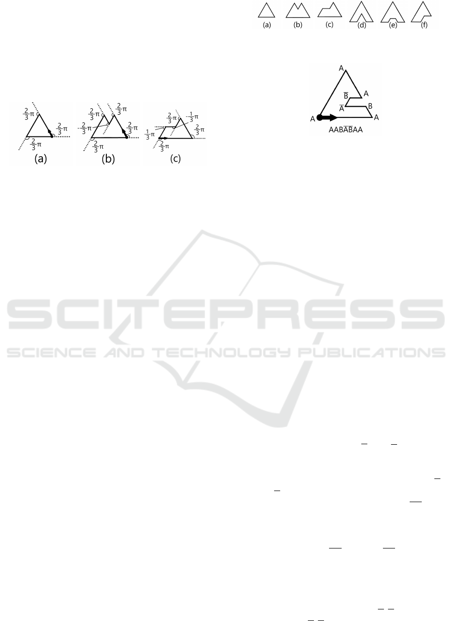
For example, the figures in Figure 1(a),(b)
and (c) are expressed as the following se-
quences: (2π/3, 2π/3,2π/3), (2π/3, 2π/3,−2π/3,
2π/3,2π/3), and (2π/3,2π/3, 2π/3,−π/3,π/3),
respectively. In the figure, the bold arrow shows the
startpoint of the sequence.
Figure 1: Angles of rotation.
It is known that the sum of the angles of rotation is
2π if and only if a closed figure can be drawn without
an intersection on a two-dimensional plane. Tosue et
al. required this proposition to define a consistency,
which is the condition to be satisfied by an expression
for the existence of a corresponding figure. However,
they did not show an algorithm that drew the figure.
In this paper, we present an algorithm that draws a
figure corresponding to the expression and present a
constructive proof of the algorithm.
We formalize the expression and the algorithm
as an abstract rewriting system (Klop, 1992). An
abstract rewriting system is generally used for dis-
cussing computational models, but can be employed
more widely to formalize a rewriting system. Here,
we define an abstract rewriting system over a set of
expressions and the rewriting rules, and present a con-
structive proof. Each rewriting rule corresponds to
the deletion of a concave part. Starting with a fig-
ure corresponding to a consistent expression, the con-
cave parts are deleted one-by-one in each step until
a simple convex shape remains. The inverse of this
procedure yields an algorithm that draws a figure cor-
responding to a given consistent expression starting
from a simple convex shape.
It is crucial to define the rewriting rules. If we try
to rewrite an edge, many possible shapes may be ob-
tained starting with a single shape. For example, con-
sider the figures shown in Figure 2. Figure (a) can be
obtained from all shapes (b)-(f) (and more) by rewrit-
ing one or two edges. It is thus essential to define rules
embracing all possible cases, but this is burdensome.
Here, we define rules for rewriting angles instead of
edges. Then, we require only four rules, which greatly
simplifies our proof.
Using this approach, the following questions
arise: (1) When a shape changes to another shape, is
there more than one sequence of rewriting steps? (2)
Figure 2: Rewriting rules.
Figure 3: Example with its corresponding expression.
For a given shape with concave parts, does the rewrit-
ing terminate, and is the given shape always rewritten
to the same convex shape?
These two questions are reduced to the principal
issues addressed by abstract rewriting systems: con-
fluence and termination. In this paper, we show that
when a shape changes to another shape, there may be
more than one sequence of rewriting steps, and for a
given shape with concave parts, rewriting terminates
at the same convex shape.
The remainder of this paper is organized as fol-
lows. In Section 2, we define our descriptive language
and rewriting system. In Section 3, we describe the al-
gorithm used to draw a figure. In Section 4, we prove
that the system exhibits confluence and termination.
In Section 5, we discuss the properties of the system.
In Section 6, we provide conclusions and describe our
planned future work.
2 LANGUAGE
Here, we define our directional language D. As ex-
plained above, D denotes figures as sequences of ro-
tational angles. We use A, B, A, and B to denote ro-
tations of 2π/3, π/3, −2π/3, and −π/3, respectively.
For example, figure (a) in Figure 1 is described by
AAA. Figures (b) and (c) are described by AAAAA
and AAABB, respectively. Another example is shown
in Figure 3; the figure is described by AABABAA.
In D, any expression denotes a closed figure. The
startpoint of the rotational sequence is irrelevant. The
use of different startpoints simply rotates the expres-
sion; for example ABABAAA or BABAAAA in Fig-
ure 3. These expressions correspond to the same fig-
ure.
The formal definition of D is as follows:
Definition 1 (Expression). An expression in D is de-
fined as a finite sequence of {A, B,A,B} (i.e., x
1
.. . x
n
where x
i
∈{A,B,A, B} for all i). We use ε to denote
Operations for Shape Transformations based on Angles
577

the empty sequence, and uv the concatenation of two
sequences u and v.
Definition 2 (Rotation). We term the function r de-
fined as r(A) = 2π/3, r(B) = π/3, r(A) = −2π/3, and
r(B) = −π/3, the rotation function. For the sequence
u = x
1
.. . x
n
, we write r(u) as Σ
n
i=1
r(x
i
).
In terms of the signs returned by the rotation func-
tion, we consider A and B (i.e., counter-clockwise ro-
tations) to be positive and
A and B (clockwise rota-
tions) to be negative rotations. Hereafter, we use x
and y for A, B, A or B, and u, v and w for sequences of
them.
Certain sequences of rotation angles cannot be
used to create closed figures. For example, BAB
should be a triangle (because it has three angles), but
the sum of the inner angles is not π, thus contradicting
an essential feature of triangles. We use the following
condition to denote (only) closed figures.
Definition 3 (Consistency). Let e be an expression of
D. If r(e) = 2π, the expression is consistent.
For the expression in Figure 3, r(AABABAA) =
r(A) ∗ 4 + r(B) + r(A) + r(B) = 2π/3 ∗ 4 + π/3 −
2π/3 −π/3 = 2π. This satisfies the consistency con-
dition. However, a question arises: Does this guaran-
tee the existence of figures corresponding to the given
expression? We answer this question in the next sec-
tion.
3 REALIZABILITY
In this section, we offer a constructive proof of re-
alizability; we develop a drawing algorithm for the
two-dimensional plane. Rewriting in D corresponds
to an operation on the figure. We consider the oper-
ation featuring addition of a convex part rather than
deletion of a concave part.
3.1 Smoothing Regions
Fundamentally, the drawing algorithm introduced in
this section seeks to smooth the smoothable regions
of a figure. Here, a “smoothable region” means a pair
of adjacent rotation angles, of which the first is nega-
tive and the second positive
1
. We write the expression
x
1
.. . x
i
x
i+1
.. . x
n
has a smoothable region at i if x
i
is
either A or B and x
i+1
is either A or B. In addition, if
1
It is possible to define a smoothable region as a pair,
of which the first is positive and the second is negative.
The characteristics can be discussed similarly, except that
smoothing can be considered as filling of concave parts in-
stead of excision.
Figure 4: Smoothing of a figure.
x
n
is either A or B and x
1
is either A or B, we write
that the expression exhibits a smoothable region at n,
and, in this case, that region is x
n
x
1
.
Definition 4 (Smoothing). Smoothing is an opera-
tion in which a smoothable region in an expression
is rewritten to become zero or one rotation angle, fol-
lowing certain rules:
1.
BA is replaced by B.
2. AB is replaced by B.
3. AA is removed (replaced by ε).
4. BB is removed (replaced by ε).
After smoothing, the expression e
0
obtained is termed
the smoothed expression of e.
For example, BABABBA is rewritten to BABBBA,
and then to BABA. This process is shown in Figure 4.
Intuitively, the operation features “excision” of the
smoothable region (the dotted line) and smoothing of
the figure.
This operation enables us to draw a figure corre-
sponding to a given expression using the figure cor-
responding to the smoothed expression. For example,
Figure 4 shows that if BABA is available, we can draw
BABBBA and BABABBA. We now prove this. For the
brevity, we skip some cases in the proof here; see Ap-
pendix for the skipped cases.
Theorem 1. Let e be a consistent expression and e
0
be the smoothed expression of e. If e
0
is drawable in
the two-dimensional plane without crossing, then so
is e.
Proof. Assume that F is the figure corresponding to
e
0
. Let d be the minimum of the distances between
two non-adjacent edges in F. From the definition, d
is less than the length of any edge. We draw the ad-
ditional edges in the region within d from F, which
makes these edges not intersect with F. We separate
the methods used to smooth e.
Case 1: When BA is replaced by B. In F, this B is
drawn as points X , Y , and Z, as shown in the following
figure. Note that in the following figures, the shaded
areas indicate the inside.
ICAART 2019 - 11th International Conference on Agents and Artificial Intelligence
578

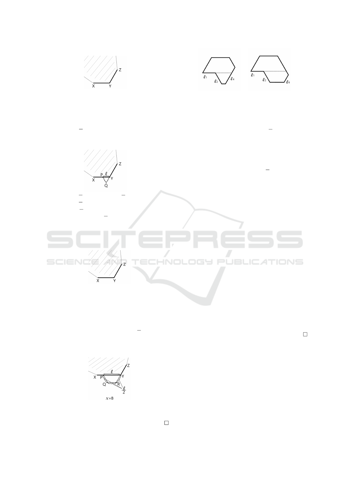
Let l be less than d. On XY , choose a point P so
that the length of PY is l. Also, choose a point Q so
that PQY is a regular triangle and Q, Y , and Z lie on
the same line. As l is less than d, PQ and QY do not
intersect with the other edges of F. The region XPQZ
corresponds to BA, and the rest is the same as e
0
. This
means that the figure is denoted by e.
Case 2: When AB is replaced by B. Skip.
Case 3: When AA is replaced by ε. Skip.
Case 4: When BB is replaced by ε. Assume that x is
the next rotation angle of BB in e. We divide the case
depending on the value of x.
• x = B: In F, x is drawn as shown below.
Let l be less than d. On XY , we place a point P so
that the length of PY is l. We create the isosceles
trapezoid PQRY ; the lengths of PQ, RY and QR
are l/2. Then, the distances between any points
on QR and the edge XY are less than d; thus, QR
also does not intersect with any other edge in F.
The region XPQRZ corresponds to BBB, and the
rest is the same as e
0
. This means that the figure is
denoted by e.
• The other cases: Skip.
Figure 5: The applicable figure (left) and the inapplicable
figure (right) of the smoothing operation.
Note that some figures are not amenable to
smoothing. For example, the two figures in Figure 5
correspond to the same expression, ABBBBBB, which
is smoothed to ABBBB. On the figure, this smoothing
should be done in a manner that we connect edge l
1
to
edge l
4
by extending l
1
, as in the left figure. However,
in the right figure, l
4
is too short to connect to l
1
. The
drawing in the above proof reveals several limitations
of the results. For example, when BBB is processed
as a part of e (see the figure in the proof in Case 4),
PQ is always shorter than RZ. This is not true in the
right figure of Figure 5; the drawing never generates
this figure.
The smoothing operation simplifies the expres-
sion, rendering it easier to draw in the two-
dimensional plane. To apply the operation repeatedly,
consistency of the expression should be preserved.
Theorem 2. Let e be a consistent expression. If e has
a smoothable region, then the smoothed expression is
also consistent.
Proof. Assume that a smoothable region at i exists in
e. In such a case, we can write e as ux
i
x
i+1
v where u =
x
1
.. . x
i−1
and v = x
i+2
.. . x
n
. When x
i
x
i+1
is replaced
by w during smoothing, the smoothed expression is
described as uwv.
As e is consistent, r(e) = 2π. From the defini-
tion of the rotation function, r(e) = r(ux
i
x
i+1
v) =
r(u) + r(x
i
) + r(x
i+1
) + r(v). For every smoothing
rule, it is easy to check that r(x
i
) + r(x
i+1
) = r(w).
Thus r(uwv) = r(u) + r(w) + r(v) = r(u) + r(x
i
) +
r(x
i+1
)+ r(v) = r(e) = 2π (i.e., the smoothed expres-
sion is consistent).
3.2 Normal Forms
We term an expression that cannot be smoothed a nor-
mal form of the expression. We prove that there are
only five normal forms in D.
Theorem 3. If a consistent expression is a normal
form (i.e., has no smoothable region), it is one of
BBBBBB, ABBBB, ABAB, AABB, or AAA, or a ro-
tation thereof.
Proof. Consistent expressions should have positive
rotations because the sum of the rotations is posi-
Operations for Shape Transformations based on Angles
579

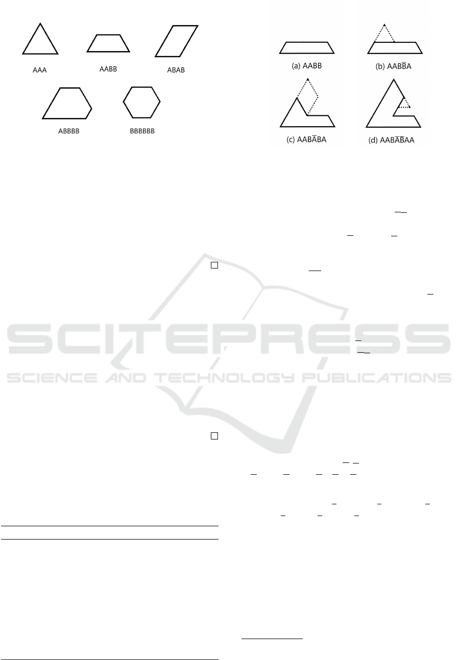
Figure 6: The normal forms.
tive (2π). If negative rotations exist, then at least
one such rotation lies adjacent to a positive rotation,
which means that a smoothable region exists. There-
fore, if e cannot be smoothed, e features only positive
rotations. Positive rotations are either π/3 or 2π/3,
and the numbers of B and A are thus (6,0), (4,1),
(2,2), or (0,3). Clearly, all of these expressions are
either of the form BBBBBB, ABBBB, ABAB, AABB,
or AAA, or a rotation thereof.
Figure 6 shows the five normal forms and this
shows that all normal forms are drawable in the two-
dimensional plane without crossing.
The last step when drawing a figure is to ensure
that the operation creates a normal form from the
given expression.
Theorem 4. For any consistent expression e, e be-
comes a normal form after a finite number of smooth-
ings.
Proof. The smoothing operation decreases the length
of any given expression; thus, after a finite number
of steps, the expression becomes an expression that
cannot be further smoothed (i.e., a normal form).
3.3 Drawing Algorithm
The following is the algorithm used to draw consis-
tent expressions. The correctness of the algorithm is
assured by reference to Theorem 1, 3 and 4.
Algorithm 1: Drawing Expression.
while smoothable region is located at i do
Push i and the shape of the smoothable region to
stack
Smooth smoothable region at i
end while
Draw normal form
while stack is not empty do
Pop the information about smoothable region
Reconstruct the smoothable region
end while
Figure 7: Drawing of the expression in Figure 3.
This algorithm shows that, for any consistent ex-
pression, there are figures in the two-dimensional
plane corresponding to the expression.
We show drawing of a figure AABABAA shown in
Figure 3. First, we find its normal form. The expres-
sion is smoothed to AABABA, AABBA, and then to
AABB, a normal form.
Next, starting from a normal form AABB, we draw
a figure for AABABAA. The process is shown in Fig-
ure 7. AABB is drawn as the trapezoid (a) in the figure.
As AABB is a smoothed expression of AABBA, we
place a regular triangle in the top left of the trapezoid
((b) in the figure). Next, we place a parallelogram on
the triangle ((c) in the figure), as the parallelogram is
a smoothable region of AABABA. Finally, we obtain a
figure corresponding to AABABAA ((d) in the figure).
We have implemented a prototype system based
on this algorithm
2
.
4 REWRITING SYSTEM
We refine the algorithm defined in the previous sec-
tion by creating a rewriting system. We use the
alphabet set Σ = {A, B,A,B} and the relation R =
{(AA,ε), (BB,ε),(AB,B), (BA,B)}.
Definition 5. S = (T,→) is a rewriting system where
T = Σ
∗
and →= {(uxyv,uwv)|uxyv ∈ T ∧(xy,w) ∈
R}∪{(yux,wu)|yux ∈T ∧(xy,w) ∈ R}.
The latter set in the definition of → enables us to
rewrite the smoothable region at the tail of expres-
sions. This is an instance of cycle rewriting of string
rewriting systems (Zantema et al., 2014) with the al-
phabet set Σ and the relation R.
We denote e → e
0
when (e,e
0
) ∈→. Also, we use
→
∗
as the reflexive-transitive closure of →.
This system has several useful properties. Here,
we prove the confluence of rewriting and the presence
2
https://ist.ksc.kwansei.ac.jp/
∼
ktaka/QSRDrawer/
RotationApplication.jar
ICAART 2019 - 11th International Conference on Agents and Artificial Intelligence
580

of a uniquely normalizing property.
Theorem 5. The rewriting system S exhibits conflu-
ence. In other words, for any expression e ∈T , if there
exist two expressions e
1
and e
2
such that e →
∗
e
1
and
e →
∗
e
2
, then there exists e
3
such that e
1
→
∗
e
3
and
e
2
→
∗
e
3
Proof. The general confluence property is derived
from the one-step confluence property (i.e., if e → e
1
and e → e
2
, then e
1
= e
2
, or e
1
→ e
3
and e
2
→ e
3
).
From the definition of R, the regions smoothed dur-
ing the transition of e to e
1
and e to e
2
are ei-
ther the same or non-overlapping. If they are the
same, clearly e
1
= e
2
. Otherwise, we can write e =
ux
1
y
1
vx
2
y
2
w, e
1
= uw
1
vx
2
y
2
w, and e
2
= ux
1
y
1
vw
2
w,
where (x
1
y
1
,w
1
),(x
2
y
2
,w
2
) ∈ R. Then, it is clear that
e
3
= uw
1
vw
2
w and e
1
→ e
3
and e
2
→ e
3
. Therefore,
the system exhibits one-step confluence, and is thus
confluent.
The confluence property is used to derive the fol-
lowing theorem.
Theorem 6. The rewriting system S exhibits a
uniquely normalizing property. In other words, for
any expression e ∈T , there is at most one normal form
e
0
such that e →
∗
e
0
.
The system S exhibits a termination property, as
revealed by Theorem 4. This means that every ex-
pression e has exactly one normal form. We discuss
classification based on normal forms in Section 5.2.
5 DISCUSSION
We discuss some properties of our rewriting system.
5.1 Symmetric Expression
Definition 6 (Symmetric). Let e
1
and e
2
be expres-
sions in D. If e
1
= x
1
.. . x
n
and e
2
= x
n
.. . x
1
, they are
said to be symmetric. It is also said that e
2
is sym-
metric to e
1
, denoted by sym(e
1
).
Clearly, if e is consistent, then sym(e) is consis-
tent.
The relevant question is whether symmetric ex-
pressions have the same normal form; the answer is
no.
Proposition 1. When expressions e
1
and e
2
are sym-
metric, their normal forms are not always the same.
We give some examples.
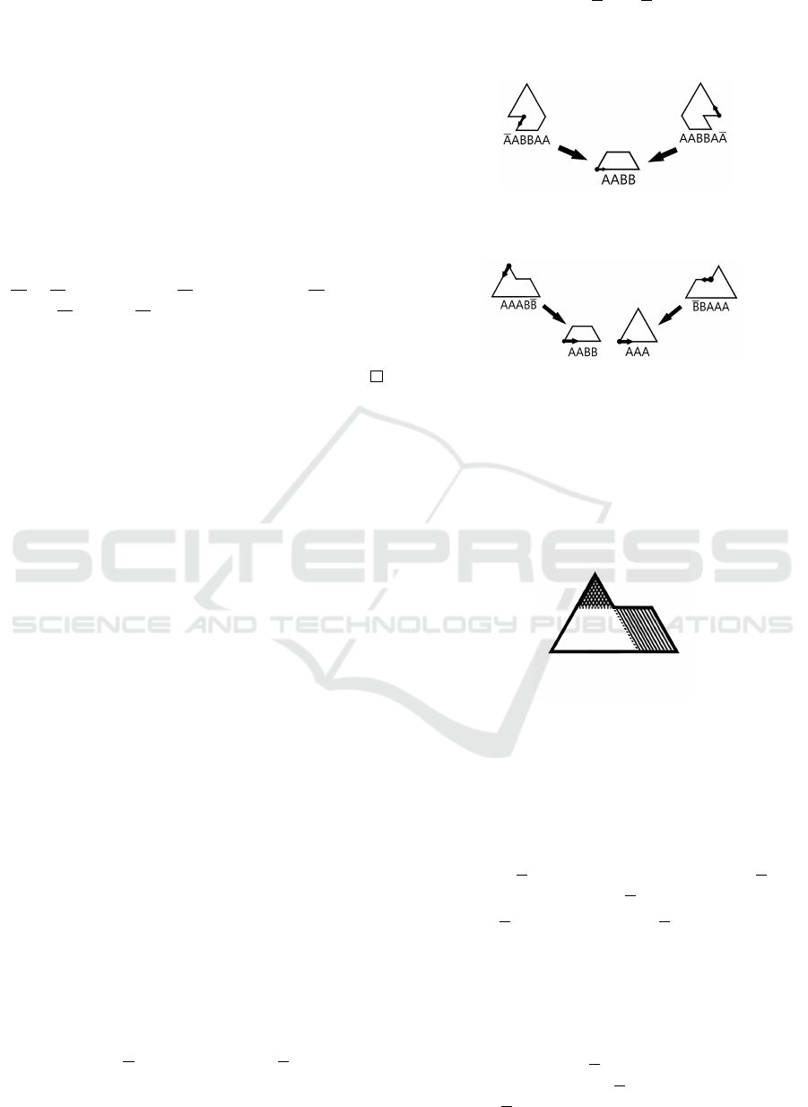
• (Example 1) AABBAA and AABBAA are symmet-
ric and have the same normal form AABB (Fig-
ure 8).
• (Example 2) AAABB and BBAAA are symmetric
but have different normal forms: AABB and AAA,
respectively (Figure 9).
Figure 8: Symmetric expressions with the same normal
form.
Figure 9: Symmetric expressions with different normal
forms.
In Example 2, we recognize two candidate
smoothable regions that are to be excised (hatched ar-
eas in Figure 10). In fact, we determine such candi-
dates by tracing the outline counter-clockwise. This
is why the symmetric expressions may have different
normal forms.
Figure 10: Candidate smoothable regions for excision.
The following proposition holds when symmetric
expressions have the same normal form.
Proposition 2. Let e = x
1
.. . x
n
(n ≥3) be a consistent
expression in D, and let e
0
be its symmetric expres-
sion. For each x
i
(i = 1,... , n), if the following two
conditions hold, then e and e
0
have the same normal
form.
1. if x
i
= A, then either x
i−1
x
i
x
i+1
= AAA or
x
i−2
x
i−1
x
i
x
i+1
x
i+2
= BBABB.
2. if x
i
= B, then x
i−1
x
i
x
i+1
= BBB.
Proof. First, we prove that symmetricity is preserved
during each rewriting for all cases.
Let u and v be x
1
.. . x
i−2
and x
i+2
.. . x
n
, respec-
tively, and also let w and z be x
1
.. . x
i−3
and x
i+3
.. . x
n
,
respectively.
Case 1: x
i−1
x
i
x
i+1
= AAA
The expression e is uAAAv, and the expression e
0
is sym(v)AAAsym(u).
Operations for Shape Transformations based on Angles
581

The expression e is rewritten to e
1
= uAv, and
e
0
is rewritten to e
0
1
= sym(v)Asym(u) by applying
the same rewriting rule. Note that if u = u
0
AA, then
e
1
= u
0
AAAv; the condition holds after the rewriting.
Therefore, e
0
1
is a symmetric expression of e
1
.
Case 2: x
i−2
x
i−1
x
i
x
i+1
x
i+2
= BBABB
The expression e is wBBABBz, and the expression
e
0
is sym(z)BBABBsym(w).
The expression e is rewritten to e
1
= wBBBBz, and
e
0
is rewritten to e
0
1
= sym(z)BBBBsym(w) by apply-
ing the same rewriting rule.
The expression e
1
is rewritten to e
2
= wBBz, and
e
0
1
is rewritten to e
0
2
= sym(z)BBsym(w) by applying
the same rewriting rule. Therefore, e
0
2
is a symmetric
expression of e
2
.
Case 3: x
i−1
x
i
x
i+1
= BBB
As in Case 1, e
0
1
is a symmetric expression of e
1
.
Therefore, symmetry is preserved during each
rewriting.
If we repeatedly apply the same rewriting rules to
these symmetric expressions, e and e
0
are reduced to
the normal forms that are symmetric. The symmetric
expression of a normal form is itself. Therefore, e and
e
0
have the same normal form.
5.2 Features of Each Class
Our rewriting system can be regarded as a state tran-
sition system in which each state denotes a shape and
each transition denotes the generation/deletion of a
concavity. From such a viewpoint, our rewriting rule
is not intuitive. For example, consider Figure 11. It
is natural to think that a figure (a) would result from
transformation of a figure (d). However, a figure (a)
can be obtained only by starting with (c) and chang-
ing through (b). It is interesting to note that similar
shapes may be obtained when the initial states differ.
Figure 11: Shape change as a state transition system.
Let e
1
and e
2
be consistent expressions in D . If e
1
and e
2
are reduced to different normal forms, then e
1
is not reduced to e
2
and vice versa. This means that
all expressions can be classified into five classes de-
pending on their normal forms. If we can extract fea-
tures that characterize each class, we can determine
the original shape of a given figure.
6 CONCLUSION
We proposed a symbolic expression for a qualitative
shape of an object in the sequence of rotation an-
gles of edges. We developed a drawing algorithm for
the expression based on rewriting strings and proved
that, for a consistent expression, it is possible to draw
a figure in the two-dimensional plane. The signifi-
cant point is that we can allocate the vertex so that
there is no intersection on the concave part. We re-
fined the algorithm as an abstract rewriting system
and proved that the system has both properties of con-
fluence and termination. The contributions of this
work are twofold:
• We offer a constructive proof for the existence of
a figure corresponding to a symbolic expression.
• We treat spatial data as an abstract rewriting sys-
tem.
There are several open problems including those
mentioned in Section 5. Of these, we are currently
considering the following:
• We are exploring other properties of the expres-
sions such as features of a set of expressions that
have the same normal form.
• We aim to provide a mechanical proof of conflu-
ence and termination using proof assistants such
as Coq and Isabelle/HOL.
ACKNOWLEDGMENT
This work was supported by JSPS KAKENHI Grant
Number JP18K11453.
REFERENCES
Cohn, A. G. (1995). A hierarchical representation of quali-
tative shape based on connection and convexity. Spa-
tial Information Theory. Cognitive and Computational
Foundations of Geographic Information Science, In-
ternational Conference COSIT’99, pages 311–326.
Galton, A. and Meathrel, R. (1999). Qualitative outline the-
ory. Proceedings of the Sixteenth International Joint
Conference on Artificial Intelligence, pages 1061–
1066.
Gottfried, B. (2003). Tripartite line tracks qualitative cur-
vature information. Proceedings of the Spatial Infor-
mation Theory. Foundations of Geographic Informa-
tion Science, International Conference, COSIT 2003,
pages 101–107.
ICAART 2019 - 11th International Conference on Agents and Artificial Intelligence
582

Gottfried, B. (2004). Reasoning about intervals in two
dimensions. Proceedings of the IEEE International
Conference on Systems, Man and Cybernetics, pages
5324–5332.
Klop, J. W. (1992). Term rewriting systems. In et al., S. A.,
editor, Handbook of Logic in Computer Science, Vol.2.
Oxford University Press.
Kulik, L. and Egenhofer, M. J. (2003). Linearized ter-
rain: languages for silhouette representations. Spatial
Information Theory. Foundations of Geographic In-
formation Science, International Conference, COSIT
2003, pages 118–135.
Leyton, M. (1988). A process-grammar for shape. Artificial
Intelligence, 34:213–247.
Ligozat, G. (2011). Qualitative Spatial and Temporal Rea-
soning. Wiley.
Museros, L. and Escrig, M. T. (2004). A qualitative the-
ory for shape representation and matching for design.
Proceedings of the Sixteenth Eureopean Conference
on Artificial Intelligence, ECAI’2004, including Pres-
tigious Applicants of Intelligent Systems, PAIS 2004,
pages 858–862.
Schlieder, C. (1996). Qualitative shape representation.
Geographic Objects with Indeterminate Boundaries,
pages 123–140.
Tosue, M., Moriguchi, S., and Takahashi, K. (2018). Qual-
itative shape representation and reasoning based on
concavity and tangent point. In Proceedings of the
31st International Workshop on Qualitative Reason-
ing.
Zantema, H., Koenig, B., and Brugging, H. J. S. (2014).
Termination of cycle rewriting. Proceedings of Joint
International Conference, RTA-TLCA 2014, pages
476–490.
APPENDIX
Proof of Theorem 1. Assume that F is the figure corre-
sponding to e
0
. Let d be the minimum of the distances
between two non-adjacent edges in F. We separate
the methods used to smooth e.
Case 1: When BA is replaced by B. Already proven
in Section 3.1.
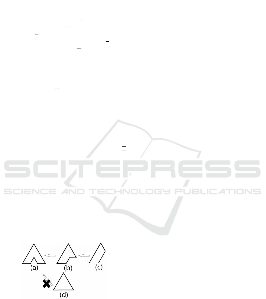
Case 2: When AB is replaced by B. Assume that x
is the next rotation angle of AB in e. In F, this Bx is
drawn as points X, Y , Z, and W . We can put the points
P and Q for each case of x as shown in the following
figures.
Let l be less than d. Distances between any point
on PQ and the edge Y Z are less than d; PQ does
not intersect with the other edges in F. The region
XY PQW corresponds to ABx, and the rest part is the
same as e
0
. This means that this figure is denoted by
e.
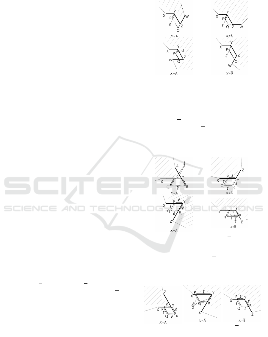
Case 3: When AA is replaced by ε. Assume that x is
the next rotation angle of AA in e. Let l be less than d,
and in the case of x = B, l be less than d/
√
3. In each
case of x, we can draw the figure in a manner similar
to the case of BBB (described in Section 3.1).
The region X PQRZ corresponds to AAx in each fig-
ure; thus, these figures are denoted by e.
Case 4: When BB is replaced by ε. Assume that x
is the next rotation angle of BB in e. We skip the
case x = B since we already proved it in Section 3.1.
For the other cases, in a manner similar to the case of
x = B, we can draw the figures as follows:
The region XPQRZ corresponds to BBx in each
figure; thus, these figures are denoted by e.
Operations for Shape Transformations based on Angles
583