Deep Neural Networks with Intersection over Union Loss for Binary
Image Segmentation
Floris van Beers, Arvid Lindstr
¨
om, Emmanuel Okafor and Marco A. Wiering
Bernoulli Institute, Department of Artificial Intelligence, University of Groningen,
Nijenborgh 9, Groningen, The Netherlands
Keywords:
Deep Learning, Image Segmentation, Loss Function, Intersection over Union, Jaccard Index.
Abstract:
In semantic segmentation tasks the Jaccard Index, or Intersection over Union (IoU), is often used as a measure
of success. While this measure is more representative than per-pixel accuracy, state-of-the-art deep neural
networks are still trained on accuracy by using Binary Cross Entropy loss. In this research, an alternative is
used where deep neural networks are trained for a segmentation task of human faces by optimizing directly
an approximation of IoU. When using this approximation, IoU becomes differentiable and can be used as
a loss function. The comparison between IoU loss and Binary Cross Entropy loss is made by testing two
deep neural network models on multiple datasets and data splits. The results show that training directly on
IoU significantly increases performance for both models compared to training on conventional Binary Cross
Entropy loss.
1 INTRODUCTION
Semantic segmentation aims to map each pixel in an
image to its associated label such as car, building
and pedestrian. In the field of image segmentation
with deep neural networks, increasingly complex sys-
tems are created to improve on the semantic segmen-
tation task. All these systems compete in complex-
ity and state-of-the-art performance. A commonality
between early works described in (Shelhamer et al.,
2017), more recent works such as SegNet (Badri-
narayanan et al., 2017) and comparative studies (Siam
et al., 2018) is that they use Intersection over Union
(IoU), also known as the Jaccard Index, as a measure
of success on test images. IoU is much more indica-
tive of success for segmentation tasks, compared to
pixel-wise accuracy, especially when the input data
is significantly sparse. When labels used for training
consist of 80-90% background, and only a small per-
centage of positive labels, a naive measure such as ac-
curacy can score up to 80-90% by labeling everything
as background. Because IoU does not concern it-
self with true negatives, this naive solution will never
occur if IoU is used as the loss function, even with
highly sparse data. While this research is focused on
binary segmentation, the naive solution problem am-
plifies itself when applied to segmentation over mul-
tiple classes as the ratio of background to a specific
class becomes worse with more classes.
With the assumption that IoU as a measure of suc-
cess is helpful, this research attempts to use a loss
function based on IoU to train a segmentation model
directly. While research has been done extensively on
which loss functions are best for which task (Janocha
and Czarnecki, 2017; Zhao et al., 2017), the default
used for image segmentation is still usually Cross En-
tropy (Shelhamer et al., 2017; Badrinarayanan et al.,
2017; Noh et al., 2015). Cross Entropy is a loss func-
tion that is, mathematically, much more closely re-
lated to accuracy than IoU, even though the final per-
formance of semantic segmentation models is mea-
sured using IoU. By defining a loss function more
closely related to IoU the training process could be
improved. As such the question that needs to be
answered is as follows: Can a model trained on an
IoU loss function perform better than a model trained
on Binary Cross Entropy (BCE) loss? Previous re-
search on optimizing IoU (Rahman and Wang, 2016)
has proposed a loss function based directly on IoU.
This loss function is tested on a single model, which
is trained on the separate classes of several semantic
segmentation datasets. Significant improvements are
found by applying this loss function to a single model.
In this research, since binary segmentation is consid-
ered, the comparison will be between this loss func-
tion based on IoU, detailed in section 2, and BCE. Op-
438
van Beers, F., Lindström, A., Okafor, E. and Wiering, M.
Deep Neural Networks with Intersection over Union Loss for Binary Image Segmentation.
DOI: 10.5220/0007347504380445
In Proceedings of the 8th International Conference on Pattern Recognition Applications and Methods (ICPRAM 2019), pages 438-445
ISBN: 978-989-758-351-3
Copyright
c
 2019 by SCITEPRESS – Science and Technology Publications, Lda. All rights reserved

timization of the IoU has also been used in other work
on semantic segmentation, as shown in work with the
Conditional Random Field (Ahmed et al., 2015) and
work on probabilistic models (Nowozin, 2014). In
another work a different loss function is proposed,
which is also based on IoU (Yuan et al., 2017). This
implementation strays further from IoU by applying a
quadratic component. As such, in this work, the loss
function without this quadratic component is used as
an implementation of IoU loss. Another loss function
proposed to optimize IoU is the Lov
´
asz-Softmax loss
(Berman and Blaschko, 2017). By using similar ar-
gumentation, this loss function was not considered in
this work due to it straying further from a purely IoU
based approach.
This research extends previous work on the topic
(Rahman and Wang, 2016), and evaluates the perfor-
mance differences between loss functions on multiple
models. In addition, to focus solely on the difference
in performance based on the loss functions, the mod-
els will use the same structure and parameters. A base
model has been created that functions when changing
the loss function, keeping all other parameters con-
stant. To further emphasize the difference in perfor-
mance based purely on the use of a new loss func-
tion a sufficiently dense dataset has been chosen. This
avoids skewing the results in favor of IoU loss, which
theoretically performs better with a sparser dataset. In
previous research (Rahman and Wang, 2016), the data
is much sparser due to the use of separate classes in
multi-class segmentation datasets, such as PASCAL
VOC2011 (Everingham et al., 2011).
In section 2, the models, datasets, and the loss
functions will be elaborated upon. Some mathemat-
ical adaptation of IoU will be used in order to make
the calculation differentiable. In section 3 the experi-
mental setup will be detailed, both in terms of hyper-
parameters and dataset splits. In section 4 the out-
come of the experiments will be presented. These re-
sults will be put into context in section 5 and evalu-
ated for statistical relevance. Furthermore, this sec-
tion shows some example output. Final conclusions
and suggestions for future work will be conveyed in
section 6.
2 METHODS
2.1 Models
In this research, two different encoders are extended
into fully convolutional networks (FCNs) for their use
as a semantic segmentation model. These encoders
are the convolutional parts of VGG-16 (Simonyan and
Zisserman, 2014) and ResNet-50 (He et al., 2015).
We have trained our own custom neural network
systems using pretrained weights from the earlier
mentioned neural network systems. These were pre-
viously trained on the ImageNet dataset (Deng et al.,
2009). The training of the custom systems employs
face images from two separate face datasets used as
input to the proposed methods. All experiments were
carried out with the aid of the Keras deep learning
framework (Chollet et al., 2015), because it contains
rich libraries for computer vision tasks.
2.1.1 VGG-16/BFCN-32s
The VGG-16 network (Simonyan and Zisserman,
2014) is a well-established deep neural network
(DNN) used for classification. It is a convolutional
network with 16 convolutional layers after which
there are several fully connected layers. Finally,
a softmax layer determines the classification out-
come. It has been trained extensively on the ImageNet
dataset (Deng et al., 2009). VGG-16 has previously
been extended to a fully convolutional network (Shel-
hamer et al., 2017). For this research the same exten-
sion from VGG-16 to FCN-32s was used as described
in previous work (Shelhamer et al., 2017). A notable
difference is the number of output classes. Where the
original FCN-32s is modelled to segment 21 classes,
i.e. the 20 classes of the VOC-2011 dataset (Evering-
ham et al., 2011) and background, the adaptation used
here considers only 2 classes. These classes are face
and background.
The main steps in adapting VGG-16 to the seg-
mentation task remain the same as described in pre-
vious work (Shelhamer et al., 2017). The fully con-
nected layers of VGG-16 are replaced with fully con-
nected convolutional layers. The first of these convo-
lutional layers has 4096 feature maps, a kernel size
of 7 × 7 and a stride of 1. This means that they are
essentially fully connected feature maps. The second
fully connected layer is replaced by a similar layer,
but with a kernel size of 1 × 1. These layers use a
rectified linear unit activation. Finally, the fully con-
nected layer that is the size of the label space is re-
placed with a fully convolutional layer with the same
purpose. This layer has 21 feature maps, one for each
class, in the original creation of FCN-32s (Shelhamer
et al., 2017) and has 1 feature map in our adaptation,
named BFCN-32s (Binary FCN-32s). This final layer
goes from feature space to label space and uses a lin-
ear activation to create the feature map.
To make the model fully convolutional, the result-
ing 7 × 7 feature maps have been upsampled by a
trainable deconvolution layer. This layer uses a stride
Deep Neural Networks with Intersection over Union Loss for Binary Image Segmentation
439

of 32 to regain the original image size and counteracts
the size decreases performed by the max-pooling lay-
ers done in each convolutional block of the encoder.
Since the number of classes is reduced to 2, a soft-
max layer as used in the original model (Shelhamer
et al., 2017) is no longer necessary. Instead, the up-
sampling layer uses a sigmoid activation to map the
output pixels to values between 0 and 1. These steps
create a model where the input image is the same size
as the output image, allowing the model to be trained
pixel-wise end-to-end.
As with the implementation of FCN-32s (Shel-
hamer et al., 2017), all layers of the VGG encoder
were frozen before training on any new data, with the
exception of the last convolutional layers positioned
in convolutional block 5. This is done to speed up the
training process. In addition, the size of the datasets
used would not influence earlier layers which are al-
ready sufficiently trained on ImageNet (Deng et al.,
2009).
2.1.2 ResNet/FCResNet
Another well-performing classification network is
ResNet-50 (He et al., 2015). This model uses resid-
ual learning in a 50-layer DNN to classify images. It
has been trained on the ImageNet dataset (Deng et al.,
2009). The same steps as described in section 2.1.1
were taken to make a fully convolutional version from
ResNet, named FCResNet in this research. While
ResNet does not have fully-connected layers, but only
a softmax layer the size of the label space, a fully con-
nected convolutional layer was added. After this a
convolutional layer was used to replace the softmax
layer and perform the same conversion from feature
space to label space as mentioned in section 2.1.1.
The fully connected convolutional layer, as described
in section 2.1.1, is used to facilitate the transition be-
tween the feature extraction part of the model and the
reduction to label space. Without this layer, the re-
duction to label space is too aggressive and therefore
loses a lot of information. This fully connected con-
volutional layer is similar to the one used in BFCN-
32s and uses 4096 feature maps, a kernel size of 7
× 7 and a stride of 1. The convolution layer replac-
ing the softmax layer reduces the feature maps from
4096 to 1 through linear activations. Finally, a similar
up-sampling layer was added to obtain an output im-
age with the same size as the input image, resulting in
a pixel-wise end-to-end trainable version of ResNet.
This up-sampling layer uses a sigmoid activation, as
explained in section 2.1.1.
As with BFCN-32s, some layers of FCResNet
were frozen. Using the same argumentation as in sec-
tion 2.1.1, all layers of the encoder were frozen except
the last convolutional block, named res5.
2.2 Datasets
To explore the differences in performance from these
models two pixel-wise labeled datasets have been
used. These are the Labeled Faces in the Wild: Part
Labels dataset (LFW) (Kae et al., 2013) and the HE-
LEN dataset (Le et al., 2012). Both sets have been
chosen for their relatively dense appearance of posi-
tive labels. The objective is to use densely distributed
data instead of sparse, because the latter might skew
the results in favor of an IoU approach, as explained
in section 1.
2.2.1 LFW
Labeled Faces in the Wild: Part Labels (Kae et al.,
2013) is a dataset containing 2927 images of faces, an
example of which is shown in figure 1. These images
are labeled in two ways, but for this research, only the
pixel-wise labeling is considered, as seen in figure 2.
This labeling is in three classes, namely face, hair and
background. Since the task considered is binary seg-
mentation, some preprocessing had to be performed.
For different experimental settings, we consider the
hair to be either part of the face, as shown in figure
3 or not, as shown in figure 4. This results in a bi-
nary labeling. The data was split by using 292 im-
ages (10%) for testing. The amount of training and
validation images are dependent on the experimental
settings as detailed in section 3.
Figure 1: Example Input Image LFW.
2.2.2 HELEN
The HELEN dataset (Le et al., 2012) is also a dataset
of faces, containing 2330 images. It is labeled in mul-
tiple classes for separate parts of the face, such as
mouth and hair. As with LFW this dataset has to be
ICPRAM 2019 - 8th International Conference on Pattern Recognition Applications and Methods
440

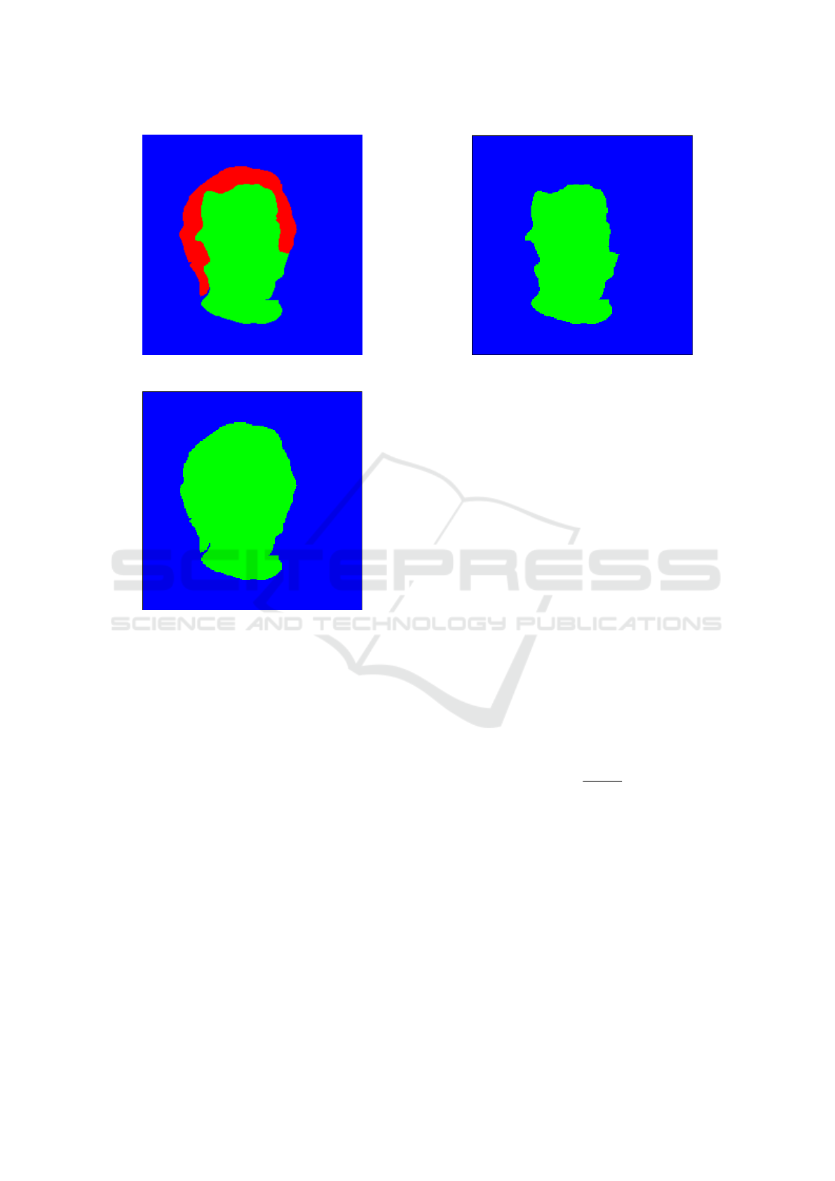
Figure 2: Example 3-class Label LFW.
Figure 3: Example LFW label with hair.
preprocessed in such a way that it can be used for bi-
nary image segmentation. As such we construct new
labels out of the provided labels that either label all
parts of the face as face and the rest as background,
or label the hair as background as well. This results
in the same data structure as with the LFW dataset.
With this dataset, 233 images (10%) are used for test-
ing. The amount of images for training and validation
are dependent on the experimental setup.
2.3 Loss Functions
In assessing the effectiveness of an IoU loss function,
a baseline has to be established. Binary Cross Entropy
(BCE) loss, or log loss, is such a baseline in that it is
used by default in a wide range of recent classifica-
tion and segmentation works (Shelhamer et al., 2017;
Badrinarayanan et al., 2017; Siam et al., 2018; Noh
et al., 2015).
The formula for binary cross entropy loss can be
seen in equation 1. In this equation T refers to the true
label image, T
x
refers to a single element of that label,
P refers to the prediction of the output image and P
x
Figure 4: Example LFW label without hair.
to a single element of that prediction.
L
BCE
=
∑
x
−(T
x
logP
x
+ (1 − T
x
)log(1 − P
x
)) (1)
The cases of P
x
= 1 and P
x
= 0 would lead to
log(0), which is undefined. To prevent this, the values
from P are clipped in the range [ε, 1 − ε]. This is done
by the Keras framework, where ε is set to 1 × 10
−7
.
In equation 1, it can be seen that BCE, while incorpo-
rating an element of probability, smoothed out by the
log component, awards both true positives and true
negatives, while penalizing false positives and false
negatives. Referring back to the problem described
in section 1, this can lead to simplistic solutions to
segmentation when the data is significantly sparse, by
labeling all output as background.
The other loss function we use is one that directly
incorporates the value for Intersection over Union.
This loss function is proposed in previous work (Rah-
man and Wang, 2016), and this previous work de-
scribes the mathematical aspects, which will be elab-
orated upon here as well. The original equation for
IoU can be given as:
IoU =
|T ∩ P|
|T ∪ P|
(2)
As before, in equation 2, T stands for the true la-
bel image, P for the prediction of the output image
and the symbols are taken from set theory. This IoU
is then taken as the average over the entire set of pix-
els producing an IoU value between 0 and 1. These
set symbols are, however, not differentiable. To apply
these set symbols in their true form, the numbers in T
and P need to be absolute 1’s and 0’s. However, while
the label image T contains these values, the output P
contains values between 1 and 0 due to the sigmoid
activation in the final up-sampling layer of the net-
work. To solve this, an approximation of IoU can be
made using probabilities. This gives the equation for
Deep Neural Networks with Intersection over Union Loss for Binary Image Segmentation
441

this approximation IoU
0
:
IoU
0
=
|T ∗ P|
|T + P − (T ∗ P)|
=
I
U
(3)
Here T and P remain the same, but T ∗ P is the
element-wise multiplication of T and P. In the nu-
merator, this gives an approximation of Intersection
by giving the probability of P
x
when T
x
is 1 and giv-
ing 0 otherwise. As such, the intersection is highest
when P
x
is 1 wherever T
x
is 1, exactly as is to be ex-
pected. The denominator is an addition of T and P
with a deduction of the Intersection, just as in a regu-
lar calculation for the union, to mitigate the effect of
counting the intersection area twice.
After reducing IoU from set operations to arith-
metic operations, producing IoU
0
, the formula is dif-
ferentiable. As a loss function, the error needs to ap-
proach 0 when results become better. To achieve this
the loss function is defined in terms of IoU
0
as such:
L
IoU
= 1 − IoU
0
(4)
This loss L
IoU
is applied to each element in a batch
and added producing a value between 0 and batch-
size, when IoU for each sample approaches 1 or 0,
respectively. This is a loss function that can, again, be
minimized. To achieve this it needs to be differenti-
ated, which is done in the following way:
∂L
IoU
∂P
x
=
−U ∗
∂I
∂P
x
+ I ∗
∂U
∂P
x
U
2
(5)
=
−U ∗T
x
+ I ∗ (1 − T
x
)
U
2
(6)
These derivatives, and the backpropagation that
follows, are computed by the Keras framework dur-
ing training when the equation used to calculate IoU
is replaced with the differentiable approximation.
3 EXPERIMENTS
Training the models using the datasets and loss func-
tions described in section 2 is done according to cer-
tain design choices, such as hyper-parameters of the
models and dataset usage. Table 1 shows the different
splits of the datasets such that 8 distinct experimen-
tal setups are created. Applying these 8 data splits to
each combination of BFCN32-s and FCResNet, either
with BCE or IoU loss, results in 32 distinct setups, the
results of which are presented in section 4.
To ensure no other factors would influence the
outcome of these experiments, any other hyper-
parameters have been kept constant. The relevant
hyper-parameters can be seen in table 2. While
most parameters are found through a parameter sweep
based on the results from previous work (Shelhamer
et al., 2017), the patience parameter is less self-
explanatory. It determines the number of epochs with-
out improvements after which the training stops. This
is our point of convergence. As such this value is
more important for total learning time than the num-
ber of epochs, the maximum of which was never
reached.
Table 1: Different data uses: Number of images used for
training and validation is given by # training and # valida-
tion respectively. The Hair? column determines whether
hair is included in the face (yes) or in the background (no).
Dataset # Training # Validation Hair?
LFW 2342 292 yes
LFW 1000 100 yes
LFW 2342 292 no
LFW 1000 100 no
HELEN 1864 233 yes
HELEN 1000 100 yes
HELEN 1864 233 no
HELEN 1000 100 no
Table 2: Experimental parameters.
Parameter Value
Epochs 1000
Batch-size 100
Patience 20
Learning Rate 0.0001
Optimizer RMSprop
Using these data splits, models and parameters,
each of the models is trained until convergence as de-
termined by the patience parameter. After training
the model was tested on previously unseen data of
the dataset it was trained on. For both datasets this
was the last 10%, i.e. 292 images for LFW and 233
images for HELEN, as mentioned in section 2.2.
4 RESULTS
The results of the experiments described in section
3 can be seen in tables 3, 4, 5 and 6. These ta-
bles are each structured similarly. Each table displays
the results of a different combination of model and
dataset and presents each of the 4 data splits within
that dataset. Results are evaluated on three metrics:
original binary accuracy, Intersection over Union and
epochs before convergence. For each metric, the re-
sults from the models trained on IoU loss are in the
L
IoU
column and the results from binary cross entropy
loss are in the L
BCE
column. Better performances are
ICPRAM 2019 - 8th International Conference on Pattern Recognition Applications and Methods
442

Table 3: Results from BFCN-32s trained and tested on LFW: The name describes whether that setting used all of the training
and validation images (big) or only 1000 training images and 100 validation images (small) and whether hair is included as
part of the face (hair) or not (no hair). Accuracy refers to the pixel-wise accuracy score for that setting. Time needed for
convergence is measured in epochs. Columns marked L
IoU
show results for IoU loss. Columns marked L
BCE
show results for
binary cross entropy loss.
Name Accuracy IoU-Score Convergence
L
IoU
L
BCE
L
IoU
L
BCE
L
IoU
L
BCE
big, hair 0.974 0.978 0.921 0.906 91 146
small, hair 0.962 0.963 0.887 0.857 116 98
big, no hair 0.977 0.976 0.896 0.852 89 83
small, no hair 0.970 0.967 0.872 0.837 155 117
Table 4: Results from BFCN-32s trained and tested on HELEN: see table 3 for clarification.
Name Accuracy IoU-Score Convergence
L
IoU
L
BCE
L
IoU
L
BCE
L
IoU
L
BCE
big, hair 0.961 0.961 0.877 0.838 125 130
small, hair 0.943 0.940 0.820 0.779 118 131
big, no hair 0.983 0.984 0.905 0.877 83 125
small, no hair 0.978 0.977 0.871 0.837 93 129
Table 5: Results from FCResNet trained and tested on LFW: see table 3 for clarification.
Name Accuracy IoU-Score Convergence
L
IoU
L
BCE
L
IoU
L
BCE
L
IoU
L
BCE
big, hair 0.942 0.947 0.829 0.826 75 64
small, hair 0.922 0.942 0.777 0.818 44 113
big, no hair 0.959 0.943 0.821 0.730 78 59
small, no hair 0.951 0.949 0.798 0.757 72 67
Table 6: Results from FCResNet trained and tested on HELEN: see table 3 for clarification.
Name Accuracy IoU-Score Convergence
L
IoU
L
BCE
L
IoU
L
BCE
L
IoU
L
BCE
big, hair 0.926 0.905 0.768 0.673 62 50
small, hair 0.916 0.917 0.747 0.723 62 97
big, no hair 0.967 0.962 0.816 0.775 68 72
small, no hair 0.963 0.960 0.796 0.766 88 80
marked in bold.
These tables clearly show that while accuracy and
convergence favor both IoU and BCE seemingly at
random, the IoU-score is distinctly higher for the new
IoU loss function in almost all experimental settings.
The exact nature and significance of this improvement
will be detailed in section 5.
5 DISCUSSION
The experiments performed and the results reported
in section 4 show the patterns for the three metrics
used to compare the two loss functions. Each of these
patterns will be discussed briefly. While binary accu-
racy has been established as being less relevant as a
measure of success for a segmentation task, it is note-
worthy nonetheless to show that it does not decrease
with the use of the IoU loss function.
Binary Accuracy. As can be observed in tables 3, 4,
5 and 6, IoU-loss and BCE-loss score higher on accu-
racy in 56.25% and 37.5% of the cases, respectively.
However, whether IoU-loss or BCE-loss results in a
higher binary accuracy, the results are within 2.5%
in every comparison. A paired t-test on these values
remains inconclusive, with a p-value of 0.52, imply-
ing no significant difference between the mean per-
formance of these loss functions based on binary ac-
curacy.
Intersection over Union. Contrary to binary accu-
racy, the results for Intersection over Union show con-
sistent and significant improvements in almost all ex-
perimental settings when using IoU-loss. A paired t-
test shows that IoU-loss scores better with a p-value
of 4.7 × 10
−4
. This is undoubtedly significant. This
Deep Neural Networks with Intersection over Union Loss for Binary Image Segmentation
443

p-value is not surprising as IoU performs better in 15
out of 16 test cases. With the exception of one test
case, improvements of multiple percentage points can
be seen across the board. On average over all cases
the error margin is reduced by 17.5%.
Convergence. While the focus of this research was
on a comparison of performance of the two loss func-
tions, an improvement in training time would also be
relevant. From the results, however, it can be seen that
these training times vary wildly. A paired t-test shows
that the average training time for IoU is lower with a
p-value of 0.256. This shows that no informed con-
clusion can be drawn about either loss function con-
verging faster.
Models. When we compare the results of BFCN-
32s and the results of FCResNet, we observe that the
BFCN-32s model performs better. Although the accu-
racies obtained with the different models do not differ
very much, the IoU scores of BFCN-32s are in gen-
eral much higher. While the encoder part of FCRes-
Net is more developed than the encoder of BFCN-
32s, the performance of the decoder is worse. This is
due to the choice of only applying a single fully con-
volutional layer in FCResNet compared to two fully
convolutional layers in BFCN-32s. This choice was
based on the amount of trainable parameters that re-
sulted in adding these layers. The output of FCRes-
Net’s encoder has considerably more parameters than
the output of BFCN-32s and, as such, connecting this
to a fully convolutional layer amplifies this dispar-
ity. A second convolutional layer in FCResNet was,
therefore, not feasible and thus the results for this
model are worse than the results for BFCN-32s.
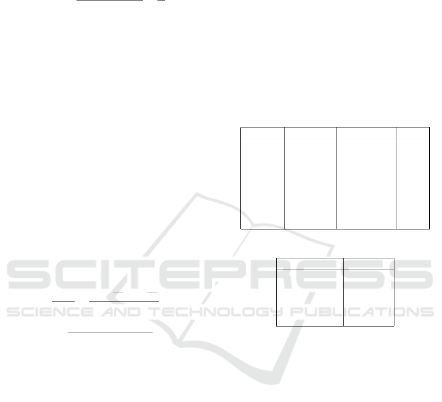
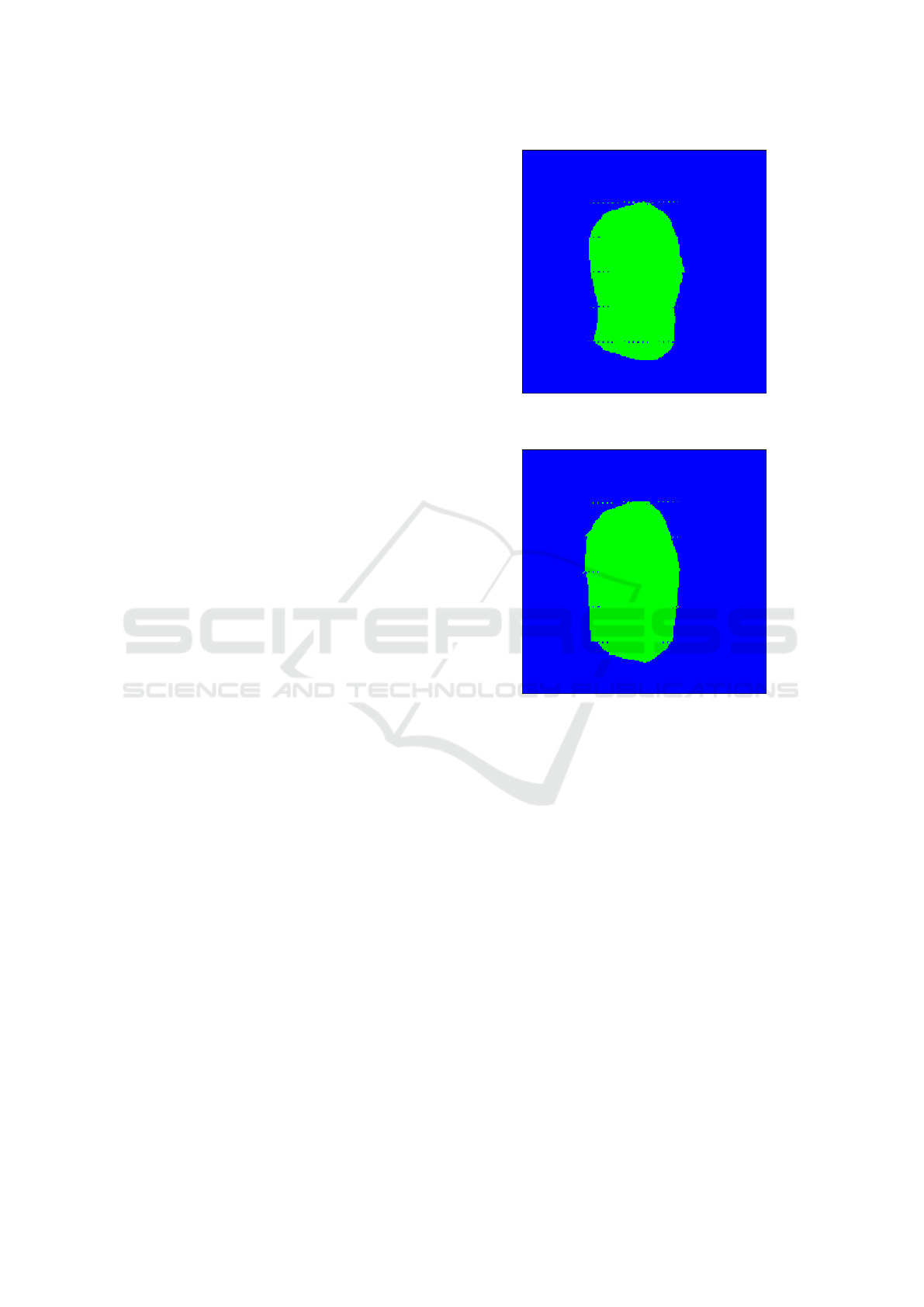
Example Output Images. In figures 5 and 6 example
outputs are shown. These images are from the exper-
imental setting using the BFCN-32s model and the
LFW dataset. They correspond to the example input
and label shown in figure 1 and figure 4, respectively.
While neither segmentation is perfect, the output for
IoU in figure 5 is clearly showing the contours of the
hairless face better than the output for BCE in figure
6. Unfortunately, for both images, some up-sampling
artifacts remain. This is most likely due to the coarse
deconvolution layer, which upsamples by a factor of
32. These up-sampling artifacts are much more pro-
nounced upon initialization and are never fully re-
moved during training.
Dataset Size. In section 3 multiple dataset splits
were described. The distinction between large and
small was made to evaluate the effect of the size of
the dataset on the effectiveness of either loss func-
tion. With the results presented in section 4 it can be
seen that whenever a smaller dataset is used, perfor-
mance suffers slightly, as is to be expected. However,
Figure 5: Example Output: BFCN-32s with IoU loss on
LFW without hair.
Figure 6: Example Output: BFCN-32s with BCE loss on
LFW without hair.
whether IoU or BCE performs better does not change
based on the size of the dataset.
6 CONCLUSION
Taking into account both the statistical analysis of the
results and the output images presented, it is clear that
training a segmentation model directly on the Inter-
section over Union objective can lead to significant
improvements. The statistical analysis shows a sig-
nificant improvement over all categories when using
IoU loss over BCE loss when the common measure
of success IoU is used. As such IoU loss is definitely
an option worth considering when attempting to im-
prove a segmentation model for state-of-the-art per-
formance. This improvement on segmentation is in
accordance with the results from previous work (Rah-
man and Wang, 2016). This research shows that these
improvements are independent of the sparsity of data.
ICPRAM 2019 - 8th International Conference on Pattern Recognition Applications and Methods
444

What is also shown by this research is that in
an ever-continuing attempt to improve state-of-the-
art Deep Neural Nets, the area of loss functions has
not been fully explored. This is in agreement with
conclusions from other work (Janocha and Czarnecki,
2017), which state that while cross entropy has been
an unquestionable favourite, adopting one of the vari-
ous other losses can be equally, if not more, effective.
These conclusions, together with the conclusion from
this and other research on the effectiveness of IoU
loss show the same thing. More and more research
is being done towards architectures, creating deeper
or different convolutional networks, while a signifi-
cant improvement can already be made by choosing a
different loss function.
While this research shows that performance im-
proves significantly for the models that were used,
this can not be claimed for every model. As such
research on IoU loss with other models, such as
the well-established SegNet (Badrinarayanan et al.,
2017), may support our hypothesis that IoU loss per-
forms better in general for semantic segmentation
tasks.
In section 1 an explanation is given why the loss
function by (Rahman and Wang, 2016) is preferred
to the loss functions proposed by (Yuan et al., 2017;
Berman and Blaschko, 2017). In future research, it is
also interesting to compare these loss functions based
on IoU directly.
Finally, the claim has been made that the bene-
fit from training on IoU directly will only magnify
when a model is presented with sparse data. This has
not been evaluated in this research and can be done
by expanding the models presented here to perform
a segmentation task on multiple classes. This would
significantly reduce the amount of positive samples in
a dataset and thus be a way to explore the hypothe-
sis that an IoU loss function outperforms binary cross
entropy on sparser data. In previous work (Rahman
and Wang, 2016) sparse data is already used. How-
ever, here the sparsity of the data is taken as it is and
not isolated to determine its effect on the performance
of the IoU loss function. As such future work could
focus specifically on certain datasets, comparing per-
formance on sparse and dense data.
REFERENCES
Ahmed, F., Tarlow, D., and Batra, D. (2015). Optimiz-
ing expected intersection-over-union with candidate-
constrained CRFs. In 2015 IEEE International Con-
ference on Computer Vision (ICCV), pages 1850–
1858.
Badrinarayanan, V., Kendall, A., and Cipolla, R. (2017).
Segnet: A deep convolutional encoder-decoder ar-
chitecture for image segmentation. IEEE Transac-
tions on Pattern Analysis and Machine Intelligence,
39(12):2481–2495.
Berman, M. and Blaschko, M. B. (2017). Optimization
of the jaccard index for image segmentation with the
Lov
´
asz Hinge. CoRR, abs/1705.08790.
Chollet, F. et al. (2015). Keras. https://keras.io.
Deng, J., Dong, W., Socher, R., Li, L. J., Li, K., and Fei-
Fei, L. (2009). ImageNet: A large-scale hierarchical
image database.
Everingham, M., Van Gool, L., Williams, C. K. I., Winn,
J., and Zisserman, A. (2011). The PASCAL Visual
Object Classes Challenge 2011 (VOC2011) Results.
He, K., Zhang, X., Ren, S., and Sun, J. (2015). Deep
residual learning for image recognition. CoRR,
abs/1512.03385.
Janocha, K. and Czarnecki, W. M. (2017). On loss func-
tions for deep neural networks in classification. CoRR,
abs/1702.05659.
Kae, A., Sohn, K., Lee, H., and Learned-Miller, E. (2013).
Augmenting CRFs with Boltzmann machine shape
priors for image labeling. In the IEEE Conference on
Computer Vision and Pattern Recognition (CVPR).
Le, V., Brandt, J., Lin, Z., Bourdev, L., and Huang, T. S.
(2012). Interactive facial feature localization. In Pro-
ceedings of the 12th European Conference on Com-
puter Vision - Volume Part III, ECCV’12, pages 679–
692, Berlin, Heidelberg. Springer-Verlag.
Noh, H., Hong, S., and Han, B. (2015). Learning de-
convolution network for semantic segmentation. In
Proceedings of the IEEE International Conference on
Computer Vision, pages 1520–1528.
Nowozin, S. (2014). Optimal decisions from probabilistic
models: The intersection-over-union case. In 2014
IEEE Conference on Computer Vision and Pattern
Recognition, pages 548–555.
Rahman, M. A. and Wang, Y. (2016). Optimizing
intersection-over-union in deep neural networks for
image segmentation. In International Symposium on
Visual Computing.
Shelhamer, E., Long, J., and Darrell, T. (2017). Fully con-
volutional networks for semantic segmentation. IEEE
Transactions on Pattern Analysis and Machine Intel-
ligence, 39(4):640–651.
Siam, M., Gamal, M., Abdel-Razek, M., Yogamani, S.,
and J
¨
agersand, M. (2018). RTSeg: Real-time se-
mantic segmentation comparative study. CoRR,
abs/1803.02758.
Simonyan, K. and Zisserman, A. (2014). Very deep con-
volutional networks for large-scale image recognition.
CoRR, abs/1409.1556.
Yuan, Y., Chao, M., and Lo, Y. C. (2017). Automatic
skin lesion segmentation using deep fully convolu-
tional networks with Jaccard distance. IEEE Trans-
actions on Medical Imaging, 36(9):1876–1886.
Zhao, H., Gallo, O., Frosio, I., and Kautz, J. (2017).
Loss functions for image restoration with neural net-
works. IEEE Transactions On Computational Imag-
ing, 3(1):47–57.
Deep Neural Networks with Intersection over Union Loss for Binary Image Segmentation
445