Overcoming Labeling Ability for Latent Positives:

Automatic Label Correction along Data Series

Azusa Sawada and Takashi Shibata

NEC Corpolation, Kanagawa, Japan

Keywords:

Machine Learning, Label Correction, Series Data, Early Detection.

Abstract:

Although recent progress in machine learning has substantially improved the accuracy of pattern recognition

and classiﬁcation task, the performances of these learned models depend on the annotation quality. Therefore,

in the real world, the accuracy of these models is limited by the labelling skills of the annotators. To tackle this

problem, we propose a novel learning framework that can obtain an accurate model by ﬁnding latent positive

samples that are often overlooked by non-skilled annotators. The key of the proposed method is to focus on

the data series that is helpful to ﬁnd the latent positive labels. The proposed method has two main interacting

components: 1) a label correction part to seek positives along data series and 2) a model training part on

modiﬁed labels. The experimental results on simulated data show that the proposed method can obtain the

same performance as supervision by oracle label and outperforms the existing method in terms of area under

the curve (AUC).

1 INTRODUCTION

In many applications such as anormaly detection for

visual inspection and medical image analysis, au-

tomation or support systems need to be developed to

reduce labor costs. To construct such systems, it is

almost necessary to use machine learning methods,

which have substantially improved the accuracy of

pattern recognition and classiﬁcation tasks. In partic-

ular, recent sophisticated models, e.g., deep convolu-

tional neural networks (Krizhevsky et al., 2012), can

achieve even better accuracy than humans.

In general, however, the performances of the mod-

els trained by such machine learning algorithms are

still limited by label quality of training data be-

cause machine learning techniques usually optimize

a model so that the model can infer assigned labels as

long as possible. For example, if positive labels are

assigned only to the absolutely positive samples (e.g.,

large tumor after critical phase), the obtained model

using this training data recognizes only the large tu-

mor. Therefore, the annotation process is absolutely

critical for the performance of the machine learning

application.

However, this annotation process usually requires

much cost, because accurate labels can be annotated

only by specialists for each application, e.g., a med-

ical specialist for cancer detection. Therefore, a ma-

𝜃

Side parameter 𝑡

Positive

Negative

Original label

“Negative”

𝑡

Corrected label

𝑡

− 𝜃

“Negative”

“Positive”

Figure 1: Concept of proposed method. Original labels are

insensitive to positives and include some overlooking. Our

method corrects labels in upper series to positive as long

as there are discriminable differences from lower series im-

ages or those remaining negative in upper series.

chine learning method is highly demanded that can

obtain an accurate model from inaccurate labels an-

notated by non-specialists.

To address this problem, we consider a way to

train models to be as sensitive to positives as they can

be without being limited by the insensitive annotation

for training datasets. In this paper, we propose a novel

framework to seek and learn latent positives missing

in negative labeled data by utilizing external informa-

tion indicating the relationship between data acquired

as a series. The concept of the proposed method is

shown in Fig. 1. Although original labels are insensi-

tive to positives, our method corrects negative labels

to positive ones for data in the upper series, which

406

Sawada, A. and Shibata, T.

Overcoming Labeling Ability for Latent Positives: Automatic Label Correction along Data Series.

DOI: 10.5220/0007341704060413

In Proceedings of the 8th International Conference on Pattern Recognition Applications and Methods (ICPRAM 2019), pages 406-413

ISBN: 978-989-758-351-3

contains original positives, as long as there are dis-

criminable differences from negatives. Our method

has two main interacting components: 1) a label cor-

rection part to seek positives along data series, and

2) a model training part on modiﬁed labels. The for-

mer process gives modiﬁed labels to the latter one,

and the latter process evaluates the separability of la-

bels from the former one by the performance of the

trained model.

Although various existing methods(Tanaka et al.,

2018) to deal with incorrect labels have been pro-

posed, these cannot ﬁnd missing positives distributed

around a class boundary because they try to correct

labels in accordance with consistency in data distri-

bution. Since most of them try to ﬁnd outliers as mis-

labeled examples, it is difﬁcult to correct consistent

labels such as pseudo labels made by other models.

Contrary to existing approaches, our idea utilizes

additional information that is effective to ﬁnd missing

positive data. Speciﬁcally, from the relationship be-

tween data acquisition conditions, we can guess posi-

tive candidates and certainly negative data. For exam-

ple, in medical diagnosis, X-lay images are captured

in the same region in the same patient on different

days. If a large tumor is found in the image taken on

the last day, a small tumor or sign of it may already

exist in previous images. This is less likely to occur

for much earlier data. In contrast, the areas labeled as

negative in last-day images are certainly also negative

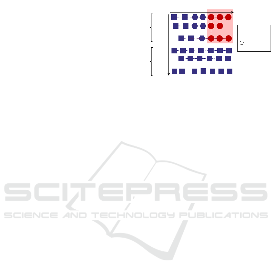
in the past images. As a generalization of this situa-

tion, we consider data acquired as series that capture

common objects under different parameters such as

time, lightning conditions, and focus levels as shown

in Figure 2. This side parameter and series ID are

also to be registered with each data. The separabil-

ity of positives from negatives increases as the side

parameter changes in each series including positives.

The proposed method tries to optimize the model

and label correction parameterized by side parameter

range, so that it satisﬁes the requirements of good per-

formance over all data and high sensitivity to latent

positives. To the best of our knowledge, this is the

ﬁrst method that can automatically correct the labels

using the property of the data series. The experiments

on two synthesized datasets show that our method can

achieve the same sensitivity as that by supervision by

oracle labels from the synthesis model, despite poor

given labels.

2 RELATED WORKS

There are many approaches to learn from dataset con-

taining wrong labels, especially related to neural net-

  

  

Side param. 

Positive series

Negative series





  

  

･･･

  

Series index 

･･･

○ Positives

□ Negatives

Latent

positives

Figure 2: Illustration of data series. Positive series are series

including positive data and negative series are series with-

out any positives. Each data has two indices: series index

and side parameter index within its series. We assume there

are hidden positives near t = t

, the side parameter value

corresponding to the ﬁrst positive in the series.

work models recently. These methods are roughly

classiﬁed into two categories: 1) robust learning un-

der label noise, and 2) label correction.

2.1 Robust Learning under Label Noise

One of the ways to deal with incorrect labels is to

surpress the inﬂuence of them. Regularlization meth-

ods are effective to learn without overﬁtting to noise

(Arpit et al., 2017; Jindal et al., 2016). The meth-

ods Backward and Forward in (Patrini et al., 2017)

modify loss function to exclude the noise effect from

optimization using an estimated label noise model by

transition matrix. As similar modeling, linear layer

to absorb noise effect is added on top of the network

architecture in (Goldberger and Ben-Reuven, 2017;

Sukhbaatar et al., 2015). There are also more explicit

treatment of noise such as (Wang et al., 2018) de-

tect outliers and assigns small weight to them. These

methods will not suit our goal because they just cancel

the noise effect without trying to learn missing posi-

tives as positive.

2.2 Label Correction

The other approach is to correct wrong label before

or during training and use it as target label. They

often require an extra dataset with ground truth of

pre-identiﬁed noisy labels to construct label clean-

ing model (Veit et al., 2017; Xiao et al., 2015; Vah-

dat, 2017). In the case that all annotators are non-

specialists, however, it is impossible to prepare such

clean dataset.

Most of works that don’t need small clean dataset

use original labels partially. Bootstrap (Reed et al.,

2015) replaces the target labels with a combination

Overcoming Labeling Ability for Latent Positives: Automatic Label Correction along Data Series

407

of raw target and their predicted labels. D2L (Ma

et al., 2018) uses local intrinsic dimensionality to de-

cide when to start using predicted labels for train-

ing and increase the weight of prediction as learning

epoch. Joint optimization (Tanaka et al., 2018) also

learn only from noisy data but it completely replace

labels by prediction learned with regularization term.

However, they cannot correct mistakes that are

easy for models to ﬁt. It is impossible to ﬁnd sam-

ples to be corrected only by data distribution in the

case of such consistent mistakes that all hard positives

labeled as negative.

Therefore, we avoid the difﬁculty in justifying the

label correction by utilizing a similarity not in feature

space but in side information such as observing con-

ditions. Note that Li et al. (2017) also utilized side

information other than the dataset, but it is only used

to regularize the learning of clean dataset to cope with

its small amount (Li et al., 2017).

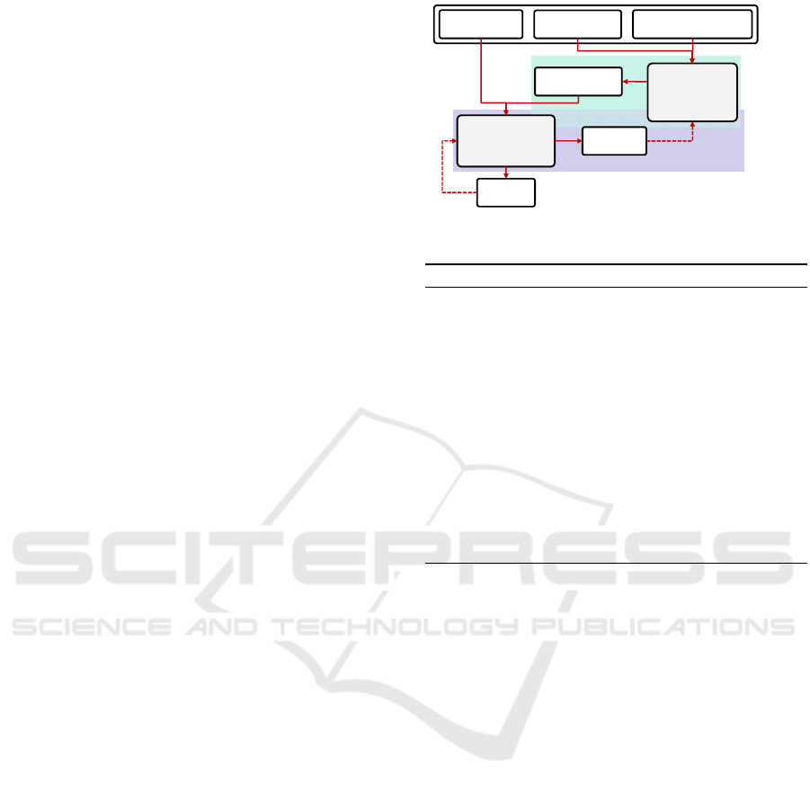
3 PROPOSED METHOD

The overview of the proposed framework is shown in

Figure 3. As explained in Sec. 1, we assume that the

training dataset consists of series with additional la-

bels, side parameter t along each series. The dataset

has data X = {X

αi

}, label Y = {Y

αi

}, and side pa-

rameter t = {t

αi

} with two indices α, i (α = 1,··· ,N.

i = 1,··· ,M

) to identify the series and the side pa-

rameter point, respectively. The proposed method

has two main interacting components: 1) label con-

troller: a label correction part to seek positives along

data series, and 2) classiﬁer: a model training part.

The classiﬁer is trained with labels modiﬁed by the la-

bel controller. The label controller recieves the train-

ing result from the classiﬁer to justify current param-

eter. In this section, the label controller and its pa-

rameterization are explained in Sec. 3.1. After that,

the concept of the optimization of label control pa-

rameter is presented in Sec. 3.2. Finally, the overall

picture and optimization procedure of our method are

described in Sec. 3.3.

3.1 Label Control along Series

We ﬁrst explain the details of the label controller that

can seek the latent positives along data series.

Missing positive data can be found in negatives

from positive series, and this is more likely to happen

if their side parameters are close to those of nearby

positives as shown in Fig. 2. However, not all neg-

ative data in positive series are latent positives that

have cognitive differences from other negatives.

⇒Sec. 3.1

⇒Sec. 3.2

Classifier

Parameters 𝑤

Data 𝑿

Labels 𝒀

Label

Controller

Parameter 𝜃

Original data

Update

Side param. 𝒕

Loss ℒ

Score 𝑠

Labels 𝒀

𝜽

Justify

Figure 3: Pipeline of proposed learning framework.

Algorithm 1: Label correction function Q.

Input: t = {t

αi

|α = 1, ··· , N. i = 1, ··· , M

}

Input: Y = {Y

αi

|α = 1, ··· , N. i = 1, ··· , M

}

Input: θ //label ﬂip threshold

Output: Y

//controlled labels

← Y //initialize output

for α = 1 to N do

if Y

αM

= 1 then

← min{t

αi

|∀i s.t. Y

αi

= 1}

for all i s.t. t

αi

≥t

−θ do

)

αi

← 1 //overwrite labels as positive

end for

end if

end for

Therefore, we parameterize the label controller by

threshold θ corresponding to the threshold for the dif-

ference in t. We optimize the threshold θ to achieve

proper correction through θ,

= Q(Y, t|θ), (1)

where Q(·|θ) is a label correction function that ﬂips

the labels of data in the positive series from negative

(i.e., Y = 0) to positive (i.e., Y = 1) on the basis of the

threshold θ as shown in Algorithm 1. Deﬁning the

reference point t

of the side parameter as the min-

imum in that of the positive data in each series, the

label controller ﬂips labels of negative data that have

a side parameter t larger than t

−θ as shown in Fig.

3.2 Threshold Justiﬁcation for Label

Control

Next, we explain how we can justify the threshold θ.

We prefer large threshold θ to ﬁnd more missing pos-

itives, but too large θ lead to label ﬂip for absolute

negatives. Our method searches for the reasonable θ

by checking if θ is too large or not on the basis of the

following idea. Let us denote the set of (X,Y ) as D

and that of (X,Y

) as D

ICPRAM 2019 - 8th International Conference on Pattern Recognition Applications and Methods

408

When θ exceeds the limit where any positive cues

completely disappear from the negatives in positive

series, the class overlaps in D

will increase. There-

fore, the limit of reasonable θ enlargement can be

detected by the separability of D

such as Fisher’s

discriminant ratio, for example. Figure 4 ilustrates

the dependency of the separability on θ. When θ in-

creases from left to right, negative data next to pos-

itives change their labels to positive. As we can

see in the upper row, the data is linearly separable

only for the smallest θ. Fisher’s discriminant ratio,

i.e. inter-class variance over inner-class variance, be-

comes smaller for larger θ because positive class take

in data around nearly overlapping region.

On the other hand, the models to use may ﬁt more

complex boundaries than that selected by a given sep-

arability metric. We should choose θ that suits the

model, so that it can perform well on D

for assumed

θ. Actually, model’s performance itself reﬂects the

separability of datasets besides the expressibity of the

model. In this sense, we can use the performance

measure as an adaptive separability score.

In this paper, we use the area under curve (AUC)

of the receiver operating characteristic (ROC) curve

for the separability score s for D

. This is be-

cause AUC can fairly compare D

among different

θs, where class popularity changes.

The two rows in Fig. 4 show the comparison be-

tween two models with different expressivities. The

separability score s starts to decrease when θ becomes

too large for each model to ﬁt the decision bound-

ary. The highly expressive model in the bottom row

keeps high s for larger θ than the upper poor model,

but ﬁnally drops at the largest θ due to excessive label

ﬂip. The dependency of s to θ used for training can

be found in Fig. 6, which is discussed in Sec. 4.1.2.

3.3 Overall Procedure

Finally, we describe the overall procedure of the pro-

posed method in detail. The proposed method opti-

mizes both classiﬁcation performance and sensitivity

to positives ignored in original labels. This can be

expressed as the single minimization problem of clas-

siﬁcation risk R and the regularization term that en-

larges the threshold θ. Let f

: X → R denote the

classiﬁer model parameterized by w,

[

θ,

w] = argmin

θ,w

{R( f

) −βθ}, (2)

Note that we should properly regularize the model or

evaluate the separability metric on a validation set separated

from training data, in the case of highly expressive models

such as deep neural networks, which may ﬁt any random

labels (Zhang et al., 2017).

High

Low

s: Low

s: High

Label sensitivity to positives

s: Low

Low

Model expressivity

Figure 4: Examples of AUCs in each situation. Squares and

circles are negative and positive(or latent positive) data, re-

spectively, and color represents assigned label. Dotted lines

link data along series. If the representative power of a model

is weak, positives too difﬁcult to classify should not be cor-

rected (θ should not be too large). When the model is strong

enough, the resulting AUC is always high. Thus, we prefer

larger θ, which means higher sensitivity to positives.

where β is the hyper parameter to balance between

classiﬁcation risk R and the importance of sensitivity

expressed by the threshold θ. In this paper, a simple

linear form was employed as the regularization

term. Our method is not limited to this form and we

can select regularization term corresponding to the

priority of accuracy or sensitivity. To obtain

θ and

we employ an alternating optimization approach by

splitting θ update and w update processes.

θ Updating Process: In the optimization of only θ,

we compare risk R before and after a label control.

Note that the minimization of the risk R corresponds

to the maximization of the performance, which can be

regarded as separability score s as described in Sec.

3.2. This optimization for θ is then expressed as fol-

lows:

θ = argmin

{R( f

) −βθ}, (3)

⇒ argmax

{s( f

) + βθ}. (4)

Since label correction is discontinuous, a simple im-

plementation of this optimization is a grid search.

Here, we assume that original labels are separable

enough for the model to lead to satisfying perfor-

mance. The separability s for the learned model will

start to drop after θ exceeds the separable limit, when

the label control threshold θ increases. In addition,

when starting from small θ, the learning process can

be seen as curriculum learning staarting from discrim-

ination of only easier positives when we use neural

network models and ﬁne-tune them in each step.

Overcoming Labeling Ability for Latent Positives: Automatic Label Correction along Data Series

409

Hence in the proposed method, we increase θ on

the grid and stop if the evaluated risk becomes higher

for temporally optimized w. Then we tune the model

again on the labels corrected by the best θ.

w Updating Process: On the other hand, if θ is ﬁxed,

the optimization of w is the standard supervised learn-

ing on corrected labels.

w = argmin

R( f

). (5)

The risk R can be altered by loss function L if you

need to realize this optimization. In our experiment,

we use the cross entropy loss with coefﬁcients in-

versely proportional to class population ratio.

3.3.1 Implementation Details

We set the initial θ as 0, which corresponds to the

original label, and increment it in accordance with a

given grid. In each step, we evaluate the separabil-

ity s on training data, which actually can be altered

by a separated validation set to prevent overﬁtting, af-

ter training on the labels controlled with current θ. If

the objective is smaller than that in the previous step,

the previous value of θ is adopted as reasonable, and

the threshold search is ﬁnished. As a result, the over-

all procedure of our method is shown in Algorithm 2.

The parameter γ, which is slightly smaller than 1, is

introduced to make the stopping condition robust to

the probabilistic deviation in s.

4 EXPERIMENTS

To evaluate the performance of the proposed frame-

work, we generated two types of synthetic datasets .

In the ﬁrst set in Sec. 4.1, we demonstrate the com-

prehensive results in simpliﬁed settings. The second

in Sec. 4.2 is a dataset of rather realistic images to

evaluate the effectiveness of our method and difﬁculty

for a related work.

4.1 Demonstration on Simple Example

First, we generated point data in two-dimensional

(2D) feature space as a simple example. We con-

ducted demonstrative experiments with the dataset

and Random Forest (Breiman, 2001), which is a com-

monly used classiﬁer for pattern recognition tasks.

4.1.1 Synthetic 2-D Point Dataset

The synthetic data model was designed to simply rep-

resent our assumption for the dataset structure shown

Algorithm 2: Learning by proposed method.

Input: X = {X

αi

|α = 1, ··· , N. i = 1, ··· , M

}

Input: t = {t

αi

|α = 1, ··· , N. i = 1, ··· , M

}

Input: Y = {Y

αi

|α = 1, ··· , N. i = 1, ··· , M

}

Input: w // initial model parameters

Input: binary classiﬁer f

: X → R

Input: θ

grid

//grid for θ search

Input: β, γ //hyperparameters for optimization

Output: f

,θ //trained model, label correction range

be f ore

← −1

initialize objective history

for θ in θ

grid

← Q(Y, t|θ)

w ←TRAINMODEL( f

,X,Y

)

s ←EVALUATEAUC( f

,X,Y

)

if s + βθ < F

be f ore

then

θ ← θ

be f ore

break

else

be f ore

← max(γs + βθ,F

be f ore

)

be f ore

← θ

end if

end for

← Q(Y, t|θ)

w ←TRAINMODEL( f

,X,Y

)

in Fig. 2. We denote the Gaussian distribution with

mean µ and covariance matrix Σ by N (·|µ, Σ) and N-

dimensional identity matrix by I

here.

For all series α, the top data X

α0

among X =

α,i

} are sampled from the same distribution

p(X|t = 0) = N (X|0,σ

I) which models the varia-

tion of captured objects. Subsequent data in negative

series are basically the same. In contrast, in positive

series, data start to shift and separate from negative

data as a model function ρ(t). Finally, we add noise

ε to all data corresponding to observation noise mod-

eled p(ε) = N (ε|0,σ

). Resulting data distributions

for the negative and positive series are as follows:

Negativeseries : p(X|t) = N (X|0, 2σ

), (6)

Positiveseries : p(X|t) = N (X|ρ(t)v, 2σ

), (7)

where ρ(t) is the underlying positive appearance

emerging from t = τ, and shift direction v is

(2,−1)/

√

5. Parameters are set as σ = 5 ×10

−2

and

τ = 0.7. The generated dataset has 200 series with

length 24 for t = 0 to 1, half of which are positive se-

ries. We keep 20 % of them as the test set. The whole

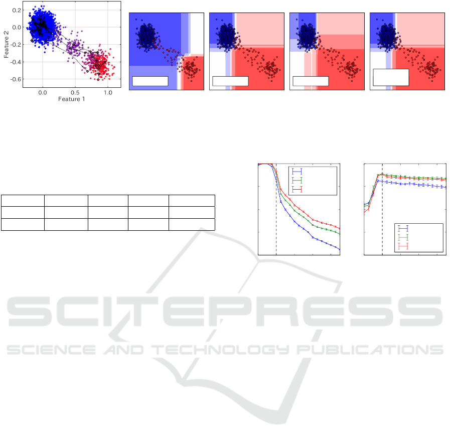
dataset is plotted in Fig. 5(a).

4.1.2 Experiment using Random Forests

In this experiment, we applied our method to a Ran-

dom Forest classiﬁer (Breiman, 2001) on 2D point

ICPRAM 2019 - 8th International Conference on Pattern Recognition Applications and Methods

410

Baseline Oracle Exceed Proposed

AUC:0.810

µ = 0

AUC:0.955

µ = 0: 2

AUC:0.933

µ = 1

AUC:0.955

µ =

µ = 0: 15

AUC:0.955

(a) 2D point data (b) Decision surface by each method

Figure 5: (a)Synthesized 2D point data. Positive series were plotted in red if labeled positive and otherwise in intermediate

color to indicate separation level. Three series are connected with dotted lines to indicate data structure. (b)Decision surface

of each method on synthesized 2D data. Plotted data are only that in test set. Each plot shows one of results for each method.

Table 1: Test performance on 2D point data for each

method. All results are averaged over 20 runs. “Acc.”

means the accuracy.

Baseline Oracle Exceed Proposed

AUC(%) 81.2(7) 95.5(3) 93.3(5) 95.4(4)

Acc.(%) 93.2(2) 95.8(2) 91(5) 95.8(3)

data described above. We compared our method

with the following three baselines that are supervised

learning using different labels: 1) Baseline: original

labels, 2) Oracle: perfect labels made by the knowl-

edge about data generation (upper limit), and 3) Ex-

ceed: labels where positive labels are extended over

all data in positive series. Original labels was made

on the assumption that annotators could ﬁnd positives

after t ≥ 0.9. In this experiment, the number of trees

is set to 8, and the depth of each tree is 3 at most.

The optimization parameters are set to γ = 0.99 and

β = 1.0. Here, each forest is trained 20 times by dif-

ferent random seeds for each method.

The results are summarized in Table 1. Figure 5(b)

shows one of resulting decision boundaries. These

results show our method has reached almost the same

performance as the oracle case in terms of AUC, with

the help of series information additional to baseline

labels. Furthermore, our method was better than the

exceed case, which also uses the series structure for

label improvement, which means the threshold search

on side information works well.

We also checked the separability score s and re-

sulting performance for each θ value to assess our

method. Figure 6 shows measured s on train data

and AUC on test data, when trained on labels con-

trolled with different thresholds θ. The evaluation of

AUC values used oracle labels for test data, and con-

troled labels for training data. We can see that AUC

decreased around the true threshold corresponding to

oracle labels for training data, and then our method

ﬁnds that point. These results show that 1) the AUC

is a suitable index for the separability score s in Sec.

3.1, and 2) the proposed procedure in Sec. 3.2 (and

0.0 0.2 0.4 0.6 0.8

Assumed threshold µ

0.6

0.7

0.8

0.9

1.0

Score s on train data

Oracle thresholdOracle thresholdOracle threshold

depth=1

depth=3

depth=5

0.0 0.2 0.4 0.6 0.8

Assumed threshold µ

0.6

0.7

0.8

0.9

1.0

AUC on test data

Oracle thresholdOracle thresholdOracle threshold

depth=1

depth=3

depth=5

Figure 6: Separability score s and performance for Random

Forests trained under label control by different thresholds

θ. The parameter depth shown in legend refers to the maxi-

mum depth of trees in Random Forests.

Algorithm 2) can correct the label so that the recogni-

tion performance becomes high on the test set with la-

bels assigned in the same criterion as the oracle case.

Note that our synthetic data are not completely sepa-

rable for oracle labels, which is why the AUC starts

to drop at a larger threshold than the true one.

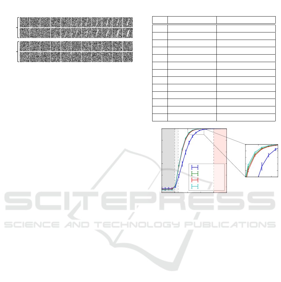
4.2 Demonstration on Realistic Dataset

For a more realistic example, we generated an image

dataset using “1” data of the MNIST handwritten digit

dataset to imitate scraches that should be detected in

a surface inspection. Positive series are designed to

represent images capturing scraches with increasing

contrast as lightening condition changes.

4.2.1 Synthetic Scratch Images with Varying

Contrast

All data in negative series share the same distribution.

Each data in negative series is noise image I

noise

gen-

erated from a simple Gaussian, which can be seen as

clean surfaces. On the other hand, the data in posi-

tive series are made by overlaying “1” images J on

noise

with the fraction of J increasing along series for

t > τ. Resulting data distributions for the negative and

Overcoming Labeling Ability for Latent Positives: Automatic Label Correction along Data Series

411

𝑡 = 0

1.00.90.1 0.2 0.3 0.50.4 0.6 0.7 0.8

Positive

series

Negative

series

Side

param.

Figure 7: Synthetic image data made by overlaying MNIST

“1” data to random noises. Upper two rows are negative

series, and the rest are positive series. The side parameter

increases from left to right and positive label is assigned to

data with t ≥ 0.8.

positive series are as follows:

Negativeseries : X(t) = I

noise

, (8)

Positiveseries : X(t) = I

noise

+ ρ(t) ·J, (9)

where ρ(t) = 0.5 ×max(0,(t −τ)(1 −τ)), 0 ≤ t ≤ 1

and τ = 0.2 in this experiment. Figure 7 shows exam-

ples generated from this model. The train set and test

set are made following the seed “1” images from the

train set and test set of MNIST dataset.

4.2.2 Experiment using CNN

Next, we evaluated our method applied to a convo-

lutional neural network (CNN) model on synthetic

scrach images.

Comparison methods are the same as in the above

experiment; 1) Baseline, 2) Oracle, and 3) Exceed.

The model used here was a simple CNN with archi-

tecture in Table 2. All convolutional layers were set to

pad=1 and stride=1 and with batch normalization be-

fore ReLU activation. The networks were trained by

momentum SGD with minibatch size 40, learning rate

0.001, moment 0.9, and weight decay 0.0005. Opti-

mization parameters of our method are set to γ = 0.99

and β = 0.2. For all methods, we ran training 20 times

using different random seeds.

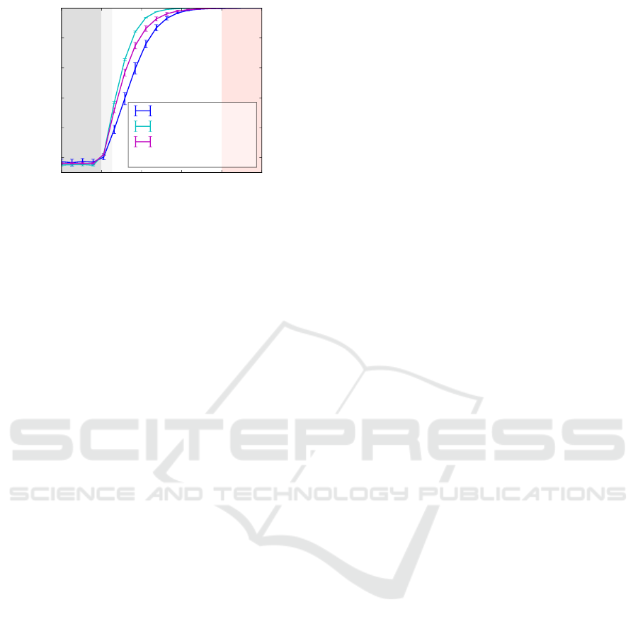
We evaluated the model trained by our method in

terms of AUC on the test set. In this experiment, we

tested AUCs at each point of a series to compare sen-

sitivities to latent positives, using test data generated

at a single fraction of J for positive series. In this eval-

uation, positive series data are all labeled as positive.

As shown in Fig. 8, our method shows high per-

formance over a wider range than the baseline. More-

over, our method achieved almost the same perfor-

mance as supervision by the oracle labels. In addi-

tion, we can see our method obtains slightly better

results even than oracle in the separable region. This

is due to the existence of overlap between class distri-

butions, and the result by the exceed was affected by

more overlaps.

Table 2: CNN architecture used in our experiment.

layer type description

in image 1 channel

1 convolution 3 ×3, 16 channels

2 convolution 3 ×3, 16 channels

pooling, dropout 2 ×2, drop ratio=0.2

3 convolution 3 ×3, 32 channels

4 convolution 3 ×3, 32 channels

pooling, dropout 2 ×2, drop ratio=0.2

5 convolution 3 ×3, 64 channels

6 convolution 3 ×3, 64 channels

pooling, dropout 2 ×2, drop ratio=0.2

7 fully connected 32 units

8 fully connected 2 units

out softmax

0.0 0.2 0.4 0.6 0.8 1.0

Side parameter t

0.5

0.6

0.7

0.8

0.9

1.0

AUC

t = t

predicted

oracle

Baseline

Oracle

Exceed

Proposed

0.4 0.5 0.6

0.95

0.96

0.97

0.98

0.99

1.00

Figure 8: AUCs on test images for proposed and baseline

methods.

4.2.3 Comparison with Existing Method

Finally, we compared the proposed method with the

existing method (Tanaka et al., 2018) that can learn

from incorrect labels, which does not use series in-

formation of the data. Figure 9 shows the existing

method result applied to base CNN used here. The

performance was better than the baseline case but not

as good as ours. This is because the existing method

modify labels not to ﬁnd latent positives but to make

decision boundary consistent. These results show

that 1) the proposed method outperforms the existing

method, and 2) the use of the series information is ef-

fective for label correction.

5 CONCLUSION

In this paper, we have proposed a learning frame-

work to overcome the limitation of model perfor-

mance by the annotating ability at preparing training

data. The proposed method utilizes the relationship

between data observing common objects and corrects

ICPRAM 2019 - 8th International Conference on Pattern Recognition Applications and Methods

412

0.0 0.2 0.4 0.6 0.8 1.0

Side parameter t

0.5

0.6

0.7

0.8

0.9

1.0

AUC

Baseline

Proposed

JointOptimization

(Tanaka+, 2018)

Figure 9: AUCs on test images compared with (Tanaka

et al., 2018). The treatment as simple label noise failed to

correct labels in the preferable way for our settings.

labels along such series. Experiments on synthesized

datasets showed that our method achieved the same

performance as supervision by oracle labels, which

is the most sensitive to positive data, not limited by

given annotation ability.

Our method enables us to get models that can ﬁnd

earlier anomalies than annotators by searching for dis-

criminative cues back to the earlier phase. In addition,

this can utilize poor labels made by simple processing

such as thresholding or by other classiﬁers.

REFERENCES

Arpit, D., Jastrzebski, S., Ballas, N., Krueger, D., Bengio,

E., Kanwal, M. S., Maharaj, T., Fischer, A., Courville,

A., Bengio, Y., and Lacoste-Julien, S. (2017). A closer

look at memorization in deep networks. In 34th Inter-

national Conference on Machine Learning (ICML).

Breiman, L. (2001). Random forests. In Machine Learning.

Goldberger, J. and Ben-Reuven, E. (2017). Training deep

neural-networks using a noise adaptation layer. In

ICLR, 5th International Conference on Learning Rep-

resentations.

Jindal, I., Nokleby, M., and Chen, X. (2016). Learning

deep networks from noisy labels with dropout regu-

larization. In 16th International Conference on Data

Mining (ICDM). IEEE.

Krizhevsky, A., Sutskever, I., and Hinton, G. E. (2012). Im-

agenet classiﬁcation with deep convolutional neural

networks. In 26th Annual Conference on Neural In-

formation Processing Systems (NIPS).

Li, Y., Yang, J., Song, Y., Cao, L., Luo, J., and Li, L.-J.

(2017). Toward robustness against label noise in train-

ing deep discriminative neural networks. In Interna-

tional Conference on Computer Vision (ICCV).

Ma, X., Wang, Y., Houle, M. E., Zhou, S., Erfani,

S. M., Xia, S.-T., Wijewickrema, S., and Bailey, J.

(2018). Dimensionality-driven learning with noisy la-

bels. IEEE.

Patrini, G., Rozza, A., Menon, A. K., Nock, R., and Qu, L.

(2017). Making deep neural networks robust to label

noise: a loss correction approach. In Computer Vision

and Pattern Recognition (CVPR).

Reed, S. E., Lee, H., Anguelov, D., Szegedy, C., Erhan, D.,

and Rabinovich, A. (2015). Training deep neural net-

works on noisy labels with bootstrapping. In ICLR, In-

ternational Conference on Learning Representations.

Sukhbaatar, S., Bruna, J., Paluri, M., Bourdev, L., and Fer-

gus, R. (2015). Training convolutional networks with

noisy labels. In ICLR, International Conference on

Learning Representations.

Tanaka, D., Ikami, D., Yamasaki, T., and Aizawa, K.

(2018). Joint optimization framework for learning

with noisy labels. In Computer Vision and Pattern

Recognition (CVPR).

Vahdat, A. (2017). Toward robustness against label noise

in training deep discriminative neural networks. In

Neural Information Processing Systems (NIPS).

Veit, A., Alldrin, N., Chechik, G., Krasin, I., Gupta, A.,

and Belongie, S. (2017). Learning from noisy large-

scale datasets with minimal supervision. In Computer

Vision and Pattern Recognition (CVPR).

Wang, Y., Liu, W., Ma, X., Bailey, J., Zha, H., Song, L.,

and Xia, S.-T. (2018). Iterative learning with open-set

noisy labels. In Computer Vision and Pattern Recog-

nition (CVPR).

Xiao, T., Xia, T., Yang, Y., Huang, C., and Wang, X. (2015).

Learning from massive noisy labeled data for image

classiﬁcation. In Computer Vision and Pattern Recog-

nition (CVPR).

Zhang, C., Bengio, S., Hardt, M., Recht, B., and Vinyals, O.

(2017). Understanding deep learning requires rethink-

ing generalization. In ICLR, International Conference

on Learning Representations.

Overcoming Labeling Ability for Latent Positives: Automatic Label Correction along Data Series

413