Distributed Range-based Localization for Swarm Robot Systems using

Sensor-fusion Technique

Daisuke Inoue, Daisuke Murai, Yasuhiro Ikuta and Hiroaki Yoshida

Toyota Central R&D Labs., Inc., Nagakute, Aichi, Japan

Keywords:

Network Localization, Swarm Robotics, Sensor Fusion.

Abstract:

Herein, we present a localization method for swarm robot systems that relies solely on measured distances

from surrounding robots. Using the sensor fusion technique, an exteroceptive estimation method based on

the measured distance is dynamically coupled with a simple proprioceptive estimation that uses a robot’s

own dynamical properties. Our method strictly preserves the locality of algorithm. The results of numerical

simulations for several scenarios show that our proposed method is more accurate that conventional methods.

1 INTRODUCTION

Swarm robot systems consist of large numbers of sim-

ple physical robots that cooperate with each other in

order to perform complicated tasks as a group (Barca

and Sekercioglu, 2013; Brambilla et al., 2013; Sahin,

2004). Recently, because such systems have attracted

signiﬁcant amounts of attention due to positive fea-

tures such as their ﬂexible adaptability to various en-

vironments and robustness against failure (Tan, 2015;

Cao et al., 1997), there has been a concurrent increase

in the proposed task execution control techniques re-

quired for such robot systems (Cheah et al., 2009;

Xie and Wang, 2007; Spears et al., 2004; Castillo

et al., 2012). In most of those control methods, each

robot is presumed to be capable of ascertaining its

own position (Wang and Guo, 2008; Bandyopadhyay

et al., 2017; Rubenstein and Shen, 2009) by means

of GPS data or via image recognition using cam-

eras installed overhead or the like. However, GPS

is limited in terms of resolution and indoor use util-

ity (Kourogi et al., 2006), and image recognition in-

volves problems in that the amount of communication

data increases along with the number of robots (Luo

et al., 2014). Therefore, in order to maximize the util-

ity of swarm robot systems, it is necessary for each

robot to be capable of estimating its own position

autonomously and locally without relying on exter-

nal systems, such as information exchanges between

swarm robots.

When discussing the behaviors of swarm robot

systems, the abilities and functions of each robot must

be ﬁxed. It should also be possible to exchange

various elements of information such as relative an-

gles, relative distances, or both (i.e., relative posi-

tions) among the robots. Of these, the use of rela-

tive distance is the most feasible because it can be

easily transmitted and received simply by installing

a single proximity sensor using infrared rays or ultra-

sonic waves on each robot body (Blais, 2004). In fact,

inexpensive robots equipped only with actuators and

a range sensor have already been developed (Ruben-

stein et al., 2012). For this reason, this study focuses

on the problem of self-position estimation from the

premise that each robot can only measure its distance

from other swarm robots. This type of problem is

called range-based localization.

Range-based localization has attracted attention in

tandem with the rapid growth of interest in swarm

robot systems and different methods have been pro-

posed to achieve it (Biswas et al., 2006; Shang et al.,

2004; Dil et al., 2006; Zhou et al., 2015; Shang and

Ruml, 2004). In (Eren et al., 2004), the geometric

conditions that a robot needs to satisfy in order to

estimate its position from distance information were

given and a position estimation method that worked

by minimizing the evaluation function of the differ-

ence between observed and estimated positions was

proposed. However, the author of (Moore et al., 2004)

pointed out that the technique in (Eren et al., 2004) is

vulnerable to observed distance noise and proposed

a more robust method in which robots ﬁrst estimate

their positions in a cluster of robots close to each

other, and then perform coordinate transformations

between clusters. We note here that in many meth-

ods, including (Eren et al., 2004; Moore et al., 2004),

Inoue, D., Murai, D., Ikuta, Y. and Yoshida, H.

Distributed Range-based Localization for Swarm Robot Systems using Sensor-fusion Technique.

DOI: 10.5220/0007258800130022

In Proceedings of the 8th International Conference on Sensor Networks (SENSORNETS 2019), pages 13-22

ISBN: 978-989-758-355-1

it is assumed that there is a so-called anchor node

that collects and calculates information of the sur-

rounding robots and then retransmits the calculated

result to the surrounding devices. This means that

as the number of robots increases, robot node com-

putational costs and memory capacity requirements

also increase, which results in communication route

congestion. To overcome this problem, in (Calaﬁore

et al., 2010), a distributed method via which a robot

could update its own estimated position simply by

communicating with the robots closest to it was pro-

posed. This method enables scalable estimations to

be performed independently of the number of robots.

In the present study, we propose a method of

range-based localization in which each robot uses in-

formation obtained both from its own dynamical char-

acteristics and relative distance measurements. More

speciﬁcally, we aim to improve the self-position es-

timation method proposed in (Calaﬁore et al., 2010)

by combining it with an estimation method based on

dynamical characteristics.

Accuracy improvements using multiple informa-

tion types has been well studied in the ﬁeld of sen-

sor fusion. For example, several methods combining

information from GPS and overhead cameras (Choi

et al., 2011; Deming, 2005; La and Sheng, 2013; Mao

et al., 2007), or applying feedback terms based on

relative distance to estimations using odometry (Mar-

tinelli et al., 2005), have been proposed. However,

in either case, the communication and calculation

costs increase as more robots are added, and scala-

bility is sacriﬁced. In contrast, in our method, the lo-

cality of the algorithm is inherited from the method

in (Calaﬁore et al., 2010) and the estimated value is

based on the dynamical model. We begin by com-

bining the two estimated values by regarding both es-

timation methods as dynamical characteristics, and

then determine the values of weights coefﬁcients in

a way that minimizes error variances. Next, after

problem formulation, we detail the algorithm proce-

dure. We also show numerical results to conﬁrm the

improvements of our proposed method over conven-

tional methods.

2 PROBLEM FORMULATION

In this section, we set up a problem for formulat-

ing the range-based localization. We begin by con-

sidering N mobile robots located on two-dimensional

(2D) space. Each robot has a unique ID from 1 to

N, and the set of these IDs is expressed as N =

{1, 2, . . . , N}. Let the states of the robot i ∈ N at

time k ∈ N be s

(k) := [x

(k) y

(k) θ

(k)]

. Here,

(k) := [x

(k) y

(k)]

∈ R

represents a point in 2D,

and θ

(k) ∈ (−π, π] represents an angle.

The purpose of this study is to provide an algo-

rithm for each robot i to use when producing a self-

position estimation ˆs

(k) = [ ˆx

(k) ˆy

(k)

(k)]

, which

should be as close as possible to its true position s

(k).

To accomplish this, we make the following assump-

tion, which is the premise of localization.

(i) The dynamics of each robot is described by the

following two-wheel vehicle model:

(k + 1) = x

(k) + εv

(k) cos(θ

(k)),

(k + 1) = y

(k) + εv

(k) sin(θ

(k)),

(k + 1) = θ

(k) + εω

(k),

(1)

where ε ∈ R

(:= {r; r ∈ R, r > 0}) is a param-

eter corresponding to the sampling period, while

(k) ∈ R and ω

(k) ∈ R represent the translation

and rotation speed of the robot, respectively.

Equation (1) represents a model in which each

robot moves in 2D space according to the input

of the translation and rotation speed. Deﬁning

input u

(k) ∈ R

as u

(k) := [v

(k) ω

(k)]

, and

g : R

× R

→ R

g(x, y) :=





+ εy

cos(x

)

+ εy

cos(x

)

+ εy





, (2)

Eq. (1) can be written as:

(k + 1) = g(s

(k), u

(k)). (3)

(ii) Since none of the robots are equipped with GPS

sensors or wheel encoders, they are incapable of

directly obtaining their true states s

(k). Hence,

it is impossible for any robot to calculate the in-

put u

(k) using state s

(k) (i.e., state feedback).

(iii) Each robot communicates with a neighboring

robot. Let us deﬁne the adjacency set N

(k), i.e.,

the set of number of robots j that can communi-

cate with robot i at time k, as:

(k) = { j ∈ N | kp

(k) − p

(k)k < D} (4)

where D ∈ R

represents the communicable

distance of the robot, and k · k represents Eu-

clidean norm: for any p ∈ R

kpk :=

p. (5)

Robot i can receive the following two pieces of

information from robot j ∈ N

(k):

(a) d

i j

(k) = kp

(k) − p

(k)k: Euclidean distance

of robots i and j,

(b) ˆp

(k): Estimated position of robot j.

SENSORNETS 2019 - 8th International Conference on Sensor Networks

(iv) In (Eren et al., 2004), the geometric conditions

that need to be satisﬁed in order to uniquely

determine a position using distance information

are shown. In that method, a network only has a

unique localization if and only if its underlying

graph is generically globally rigid. We assume

that this condition is satisﬁed at an arbitrary time

k ∈ N.

3 LOCALIZATION ALGORITHM

3.1 Proprioceptive Estimation

First, we will describe a localization method based on

the dynamical characteristics of each robot shown in

Eq. (1). Let ˜s

(k) = [ ˜x

(k) ˜y

(k)

(k)]

be the esti-

mated value of the state of robot i at time k and u

(k)

be the input, and let these be known. Then, the value

of the state at the next time ˜s

(k + 1) is estimated by

using Eq. (1) as follows:

˜s

(k + 1) = g( ˜s

(k), u

(k)).

(6)

Hereafter, the method based on Eq. (6) is called

the proprioceptive method. Unlike the exteroceptive

method detailed in the next section, since the infor-

mation necessary for the estimation is closed in each

robot, estimation accuracy does not depend on com-

munication quality with the neighboring robots. An-

other advantage is that it allows the robot to estimate

the angle, as well as its position. However, since

Eq. (6) excludes a feedback term for the observed in-

formation, errors accumulate over time and the devi-

ation from the true value eventually becomes large.

3.2 Exteroceptive Estimation based on

the Distributed Gradient Method

Here, we present a localization method based on com-

munication with neighboring robots. Suppose that

each robot i receives an observed distance value from

neighboring robot d

i j

and an estimated position of

neighboring robot ˆp

. First, we deﬁne an evaluation

function f : R

→ R that shows the consistency of

the estimated position with respect to the observed

distance:

f ( ˆp(k)) =

∑

i∈N

∑

j∈N

(k ˆp

(k) − ˆp

(k)k − d

i j

(k))

, (7)

ˆp(k) := [ ˆp

(k)

ˆp

(k)

··· ˆp

(k)

]

. (8)

The localization is then formulated as an optimization

problem that minimizes the function f :

minimize f ( ˆp(k)). (9)

One of the most common methods for solv-

ing the optimization problem above is the gradient

method (Eren et al., 2004). This method ﬁrst esti-

mates an appropriate initial position and updates the

estimated position via:

ˆp(k + 1) = ˆp(k) − α(k)∇ f ( ˆp(k)), (10)

where α(k) ∈ R

is the design parameter called a step

length. As α(k) becomes larger, the convergence of

the ˆp(k) becomes faster. However, if the value of α(k)

is too large, then ˆp(k) diverges. As a condition for

the convergence of ˆp(k), what is called a Walfe con-

dition is known. When α(k) satisﬁes this condition,

Eq. (10) converges to the local optimal solution (No-

cedal, 2006).

In Eq. (10), the gradient ∇ f depends on the esti-

mated position of all robots ˆp(k), but it consists of the

sum of the pair terms of the estimated positions that

are located in the neighborhood. Using this property,

we can decompose it and rewrite Eq. (10) for each

robot i as follows:

ˆp

(k + 1) = ˆp

(k) − α

(k)∇

( ˆp(k)), (11)

where we deﬁned f

( ˆp(k)) =

∑

j∈N

(k ˆp

(k) − ˆp

(k)k − d

i j

(k))

, (12)

and ∇

f denotes the i-th 1×2 block in the gradient ∇ f

in Eq. (10). We generalized the step length as α

(k).

By applying Eq. (11), each robot independently

updates its estimated position with a calculation of the

local evaluation function f

. This method type is often

called a distributed gradient method (Calaﬁore et al.,

2010). In this study, it is adopted as the exteroceptive

method. In order to satisfy the Walfe condition, the

author of (Calaﬁore et al., 2010) proposed a method

of sequentially updating the weights α

(k) so that the

robots could communicate. For simplicity, however,

we assume that weight α

(k) is invariant over time,

and set α as the common weight for all robots.

Since the exteroceptive method uses distances be-

tween robots, the estimation performance degrades if

the distance measurement is not accurate. In addi-

tion, since only the robot position is estimated with

this method, it is not possible to estimate the state in-

cluding the angle of the robot. To overcome these

challenges, we propose a position estimation method

that works by fusing both the proprioceptive and exte-

roceptive methods, as will be detailed in the following

section.

3.3 Proposed Estimation Method

In the previous subsections, we have shown the state

estimation algorithms using proprioceptive and exte-

roceptive information. The drawback of the former

Distributed Range-based Localization for Swarm Robot Systems using Sensor-fusion Technique

is in that it is weak against modeling errors and input

noises, while the latter is vulnerable to distance mea-

surement errors. We will now propose a new method

that improves performance by obtaining the weighted

sum from the error variances of the two estimated val-

ues.

First, we will describe error variance minimiza-

tion. Suppose that a variable z is estimated by two dif-

ferent methods as ˜z, ˆz and that the errors of the meth-

ods are deﬁned as

δ = z − ˜z,

δ = z − ˆz. Then, assuming

that the variance of

δ and

δ is calculated as

V ,

V , the

weighted sum of ˜z and ˆz,

¯z = ˜z + (

−1

)

−1

(ˆz − ˜z), (13)

is known to minimize the error variance of estimated

value (Gustafsson, 2010). In the following subsec-

tion, we evaluate the error variance of position esti-

mated using both the proprioceptive and exterocep-

tive methods and then combine the estimation values

using the Eq. (13).

3.3.1 Error Variance of Proprioceptive Method

First, we derive an approximate expression for esti-

mating the error distribution of the states in the propri-

oceptive method. The input command value for robot

i at time k is denoted as u

(k), and the input actually

applied is denoted as u

(k). We then write the input

error as δ

(k) := u

(k) − u

(k). Additionally, we de-

note the true and estimated value of the state of robot

i as s

(k) and ˜s

(k) respectively, and the estimation er-

ror as δ

(k) := s

(k) − ˜s

(k).

Then, the state at time k + 1 is represented as

(k + 1) = g(s

(k), u

(k))

= g( ˜s

(k) + δ

(k), u

(k) + δ

(k)).

(14)

By linearizing the right-hand side of Eq. (14), we ob-

tain

(k + 1) ≈ g( ˜s

(k), u

(k)) + J

(k)

(k) + J

(k)

(k),

(15)

where we have deﬁned

(k)





1 0 −ε sin(

θ(k))v

(k)

0 1 ε cos(

θ(k))v

(k)

0 0 1





, (16)

(k)





ε cos(

θ(k)) 0

ε sin(

θ(k)) 0

0 ε





. (17)

Therefore, the estimation error δ

(k + 1) caused by

Eq. (6) is written as the following expression:

(k + 1) := s

(k + 1) − ˜s

(k + 1)

= s

(k + 1) − g( ˜s

(k), u

(k))

≈ J

(k)

(k) + J

(k)

(k).

(18)

We then assume the following in order to obtain an

approximate representation of the error variance using

the above equation: (i) Estimated error of state δ

(k)

is a random variable, and its distribution is a Gaussian

distribution with an average of 0 and a variance of

(k). (ii) Similarly, let δ

(k) be a random variable

that follows the Gaussian distribution N(0,V

) at all

times k. (iii) δ

(k) and δ

(k) are independent.

Then, if we know

(0) and V

for all i ∈ N , the

error variance of state at time k + 1 is approximated

using information at time k as

(k + 1) = J

(k)

(k)J

(k)

+ J

(k)

. (19)

3.3.2 Error Variance of Exteroceptive Method

Next, we derive the error variance of state in the ex-

teroceptive method. Let d

i j

(k) be the true distance

between robots i and j at time k, let d

i j

(k) be the

observed distance, and deﬁne the error as δ

i j

(k) :=

i j

(k) − d

i j

(k). We further assume that the true and

estimated position of robot i is p

(k) and ˆp

(k) respec-

tively, and the estimation error is δ

(k) := p

(k) −

ˆp

(k).

In Eq. (11), if d

i j

(k) is correctly observed, the es-

timated value ˆp

(k) is expected to converge to the true

value p

(k) as k → ∞. In addition, if ˆp

(k) = p

(k)

holds, in the next iteration in Eq. (11), ˆp

(k + 1) =

(k + 1) is expected to hold as well. However, this is

not the case if d

i j

(k) is not correctly observed. In this

situation, the true position p

(k) is written as

(k + 1)

= p

(k) − α∇

∑

j∈N

(kp

(k) − p

(k)k − d

i j

(k))

= ˆp

(k) + δ

(k)

− α∇

∑

j∈N



k( ˆp

(k) + δ

(k)) − ( ˆp

(k) + δ

(k))k

−(d

i j

(k) + δ

i j

(k)



(20)

By linearizing the right-hand side of Eq (20), we ob-

tain

(k + 1)

= ˆp

(k) − α∇

∑

j∈N

(k ˆp

(k) − ˆp

(k)k − d

i j

(k))

+ J

(k)

(k) +

∑

j∈N

i j

(k)

(k) +

∑

j∈N

i j

(k)

i j

(k),

(21)

SENSORNETS 2019 - 8th International Conference on Sensor Networks

where we deﬁned

(k)



1 0

0 1



− α

∑

j∈N

i j

, (22)

i j

(k)

:= αP

i j

, (23)

i j





1 −

i j

(k) ˆy

i j

(k)

k ˆp

i j

(k)k

i j

(k) ˆx

i j

(k) ˆy

i j

(k)

k ˆp

i j

(k)k

i j

(k) ˆx

i j

(k) ˆy

i j

(k)

k ˆp

i j

(k)k

1 −

i j

(k) ˆx

i j

(k)

k ˆp

i j

(k)k





, (24)

i j

(k)

:= α







ˆx

i j

(k)

k ˆp

i j

(k)k

ˆy

i j

(k)

k ˆp

i j

(k)k







, (25)

ˆx

i j

(k) := ˆx

(k) − ˆx

(k), (26)

ˆy

i j

(k) := ˆy

(k) − ˆy

(k), (27)

ˆp

i j

(k) := ˆp

(k) − ˆp

(k). (28)

Therefore, the estimation error δ

(k + 1) resulting

from Eq. (11) is written as:

(k + 1)

:= p

(k + 1) − ˆp

(k + 1)

≈ J

(k)

(k) +

∑

j∈N

i j

(k)

(k) +

∑

j∈N

i j

(k)

i j

(k).

(29)

As in the previous subsection, the following as-

sumptions are made in order to obtain an approximate

representation of error variance: (i) For all i ∈ N , the

estimated error of position δ

(k) is a random vari-

able, and its distribution is Gaussian with an average

of 0 and a variance of

(k). (ii) δ

i j

(k) is also a

random variable that follows the Gaussian distribu-

tion N(0,V

i j

). (iii) δ

(k), δ

i j

(k) are independent.

Then, if we know

(0) and V

i j

for all i, j ∈ N ,

the error variance of estimated position at time k + 1

is approximated as:

(k + 1) = J

(k)

(k)J

(k)

∑

j∈N

i j

(k)J

i j

∑

j∈N

i j

(k)

i j

(k)

(30)

3.3.3 Fusion of Estimated Values

We use Eq. (13) to combine the variances in the esti-

mation methods calculated above. Note that the exte-

roceptive method only estimates the position and does

not have angle information. Therefore, let the error

variance of estimated angle be inﬁnite and deﬁne the

expanded variance

(k) as

(k) :=



(k) 0

0 ∞



. (31)

Using this, the merged estimated value ¯s(k) is given

as the following expression:

¯s

(k) = ˜s

(k)

+ (

(k)

−1

(k)

−1

)

−1

(k)

−1

( ˆs

(k) − ˜s

(k)).

(32)

4 NUMERICAL EXAMPLES

In this section, we show several numerical results for

various practical situations in order to compare the es-

timation performances of the proprioceptive method,

exteroceptive method, and a method of “fusing” the

two values.

When the position of robot i at time k is written

as p

(k) and the estimated position is written as ˜p

(k),

the following two indices are considered for evaluat-

ing the estimation quality:

(i) Function J

that represents the distance between

the estimated value and the true value:

∑

i∈N

(k) − ˆp

(k)k. (33)

(ii) Function J

representing the consistency with re-

spect to observed distance:

∑

i∈N , j∈N

|k ˆp

(k) − ˆp

(k)k − d

i j

(k)|, (34)

We also consider the mean over the calculation time,

∑

k=0

, (35)

∑

k=0

, (36)

where K ∈ N represents the termination time of the

simulation.

The parameters commonly set in this section are

as follows: We ﬁrst assume the communicable dis-

tance D is equal to 5.0. In the dynamics of the robot

Eq. (1), the sampling period ε, which should be sufﬁ-

ciently small compared to a typical velocity of robots

(in the following simulation, velocity is typically set

to 5.0), is assumed that ε = 0.01. In the exterocep-

tive method, the step length of the gradient method

is α = 0.1, which is a reasonable choice because the

typical length-scale of our system is the communica-

ble distance D. Unless otherwise stated, the following

values are used for the error variance of signal used in

Distributed Range-based Localization for Swarm Robot Systems using Sensor-fusion Technique

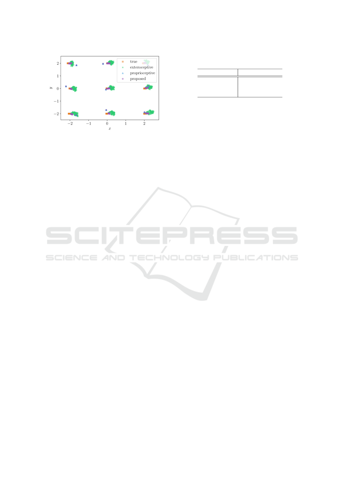
Figure 1: Trajectories of nine robots. All robots are shown

stopped at their initial position. The positions estimated by

the proposed method (purple circle) are compared to the ac-

tual location (orange square). The positions estimated by

the exteroceptive method only (green star) and the proprio-

ceptive method only (blue triangle) are also shown for com-

parison.

the fusion of the weights in the proposed method:

(0) = diag(0.09, 0.09), (37)

(0) = diag(0.09, 0.09), (38)

= diag(0.04, 0.04), (39)

i j

= 0.09, (40)

Here it should be noted that, in the numerical calcu-

lations, the white noise following the Gaussian distri-

bution whose average is 0 and whose variance is rep-

resented by Eqs. (37)-(40) is supposed to be applied

additively.

4.1 Performance in the Stationary Case

In this subsection, we report on a comparison of po-

sition estimation performance for a swarm consist-

ing of nine robots. The initial positions were set

in a lattice pattern, that is, x

(0) ∈ {−2.0, 0.0, 2.0},

(0) ∈ {−2.0, 0.0, 2.0}. The input of all robots was

set to 0:

(k) =



0.0 0.0



. (41)

Figure 1 shows the trajectory of each estimated

robot position using all three estimation methods. In

the proprioceptive method, since the initial estima-

tion state is not updated, an estimation error appears

and increases steadily. The exteroceptive method esti-

mates a value deviating from the true value due to the

inﬂuence of the observed distance error. In contrast,

the proposed method estimates values very close to

the true positions.

In Fig. 2, the time responses of the two evaluation

functions J

, J

deﬁned by Eqs. (33), (34) are shown.

Table 1: Elapsed time of 1000 step simulation in the sta-

tionary case.

Method Elapsed time [s]

proprioceptive 5.66

exteroceptive 7.23

proposed 13.84

Fig. 2 shows that the proposed method estimates po-

sitions closer to their true values than both the pro-

prioceptive and exteroceptive methods. In particular,

in Fig. 2-(a), it can be seen that the error of the ex-

teroceptive method is large, whereas the error is sup-

pressed in the proposed method. This reﬂects the pro-

prioceptive information that the robots are at rest at

their initial positions.

We have also checked the computational time

for each estimation method. Table 1 compares the

elapsed time of 1000 step simulation. It shows that

the time taken in the proposed method is almost equal

to the sum of those taken in the other two methods,

conﬁrming that the combination of the two methods

does not cause any unreasonable overhead.

4.2 Performance in the Dynamic Case

As in Sec. 4.1, nine robots are arranged in a grid

pattern. Three units of y

(0) = −2 turn to the left,

three units of y

(0) = 2 turn to the right, and three

units y

(0) = 0 remain at rest on their initial posi-

tions. Speciﬁcally, the input u

(k) to each robot is

represented by

(k) =











0.0 0.0

for y

(0) = 0,

5.0 5.0

for y

(0) = −2,

5.0 −5.0

for y

(0) = 2.

(42)

Fig. 3 shows the trajectories of each estimated robot

position obtained by the three estimation methods.

Here, it can be seen that the proposed method posi-

tion estimates are somewhat more accurate than the

other two methods. The estimated value of the pro-

prioceptive method is biased over the entire time due

to the inﬂuence of the initial error and input noise.

The exteroceptive method estimates a value deviating

from the true value because of the observed distance

error inﬂuence.

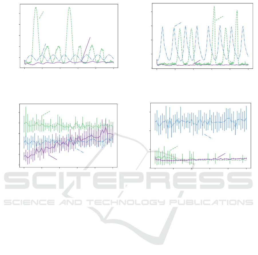
Figure 4 plots the time responses of two evalua-

tion functions J

, J

deﬁned by Eqs. (33), (34), which

again conﬁrm the accurate estimation of the proposed

method compared to both the proprioceptive and ex-

teroceptive methods.

We have also checked the computational time for

this case. Table 2 shows the elapsed time of 1000 step

SENSORNETS 2019 - 8th International Conference on Sensor Networks

0 200 400 600 800 1000

0.0

0.2

0.4

0.6

0.8

exteroceptive

proprioceptive

proposed

0 200 400 600 800 1000

0.05

0.10

0.15

0.20

0.25

0.30

0.35

exteroceptive

proprioceptive

proposed

(a) (b)

Figure 2: Histories of two evaluation functions: (a) J

, (b) J

. The value of the present method (purple solid) is compared to

that of the exteroceptive method (green dashed) and of the proprioceptive method (blue dash-dot).

Figure 3: Trajectories of nine robots. Three units of y

(0) =

−2 turn to the left, three units of y

(0) = 2 turn to the right,

and three units y

(0) = 0 remain on their initial positions.

The positions estimated by the proposed method (purple

circle) are compared to the actual location (orange square).

The positions estimated by the exteroceptive method only

(green star) and the proprioceptive method only (blue trian-

gle) are also shown for comparison.

Table 2: Elapsed time of 1000 step simulation in the dy-

namic case.

Method Elapsed time [s]

proprioceptive 5.99

exteroceptive

6.67

proposed 11.68

simulation for each estimation method. Similarly to

the previous subsection, the time taken for the pro-

posed method is about the same as the sum of the time

taken for the component methods.

4.3 Input Noise Effect

Here we examine the performance while varying

the magnitude of the standard deviation σ

diag(σ

, σ

)) of the noise applied to input u

(∀i ∈

N ). The initial positions and inputs are the same as

in Sec. 4.2.

In Fig. 5, the value of two evaluation functions

deﬁned as Eqs. (35), (36) with respect to σ

are

shown. The termination time is K = 200 unless oth-

erwise is stated.

Figure 5-(a) shows that, when σ

is small in the

proposed method, the value of Eq. (35) is also small.

However, as σ

gets larger, it approaches the value of

Eq. (35) in the exteroceptive method. This is because

of the weight adjustment function, which puts higher

weight on the exteroceptive information than on the

proprioceptive information, as the variance of the in-

put noise increases. On the other hand, in Fig. 5-(b),

the proposed method makes the evaluation function

small even when σ

is large. Thus, we can con-

clude that our proposed method gives a value that is

most consistent with the geometric relationship of all

robots.

4.4 Observation Noise Effect

Next, we investigate the impact of the applied noise

by examining the observed distance d

i j

(∀i ∈ N , j ∈

) while changing the magnitude of the standard de-

viation σ

. The initial positions and inputs are the

same as in Sec. 4.2.

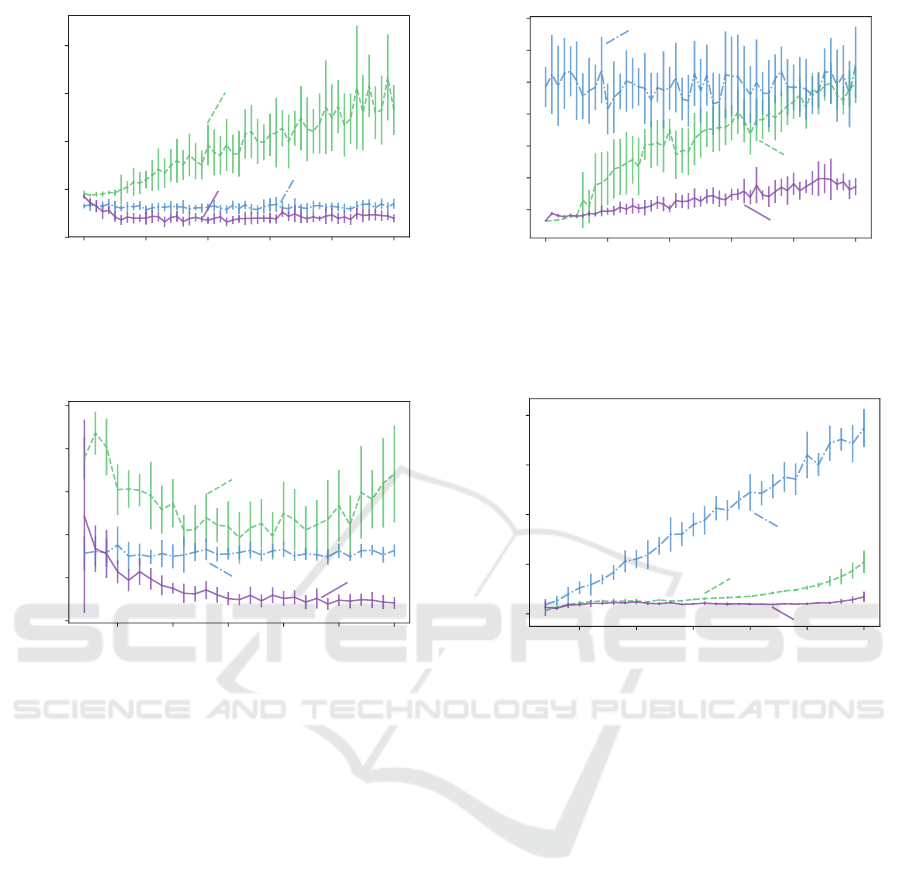
In Fig. 6, we show the value of two evaluation

functions

deﬁned by Eqs. (35), (36) with respect

to σ

. The estimation accuracy degrades as the noise

increases in the exteroceptive method. On the other

hand, in the proprioceptive and proposed methods, no

remarkable adverse effect is observed. In addition,

in Figs. 6-(a), (b), regardless of the value of σ

, the

proposed method takes a smaller value than the pro-

prioceptive estimate. These results allow us to con-

clude that the proposed method is the most robust of

the three methods against observed distance errors.

Distributed Range-based Localization for Swarm Robot Systems using Sensor-fusion Technique

0 200 400 600 800 1000

exteroceptive

proprioceptive

proposed

(a) (b)

0 200 400 600 800 1000

0.5

1.0

1.5

2.0

2.5

exteroceptive

proprioceptive

proposed

(a)

Figure 4: Histories of two evaluation functions: (a) J

, (b) J

. The value of the present method (purple solid) is compared to

that of the exteroceptive method (green dashed) and of the proprioceptive method (blue dash-dot).

0.0 0.2 0.4 0.6 0.8 1.0

exteroceptive

proprioceptive

proposed

0.0 0.2 0.4 0.6 0.8 1.0

0.1

0.2

0.3

0.4

0.5

0.6

exteroceptive

proprioceptive

proposed

(a) (b)

Figure 5: Value of two evaluation functions: (a)

, (b)

, compared with the magnitude of input noise σ

. Each line

represents the average value obtained when the numerical calculation was performed 10 times, and the length of the vertical

bar represents the standard deviation of 10 times. The value of the present method (purple solid) is compared to that of the

exteroceptive method (green dashed) and of the proprioceptive method (blue dash-dot).

4.5 Effect of the Number of Robots

Finally, we examine the effect of the number of robots

N on the estimation performance. The initial conﬁgu-

ration of the robots is generated as a uniform random

number taking a value range in (−2.5, 2.5)

. The in-

put u

(k) to each robot is deﬁned by

(k) =











0.0 0.0

for i = 3n (n ∈ N),

5.0 5.0

for i = 3n + 1 (n ∈ N),

5.0 −5.0

for i = 3n + 2 (n ∈ N).

(43)

The values of two evaluation functions

de-

ﬁned in Eqs. (35), (36) with respect to N are shown

in Fig. 7. As in Fig. 7-(a), the error of the proposed

method decreases as N increases. This accuracy im-

provement stems from the fact that each robot has

larger amounts of information for larger N. In Fig. 7-

(b),

increases as the value of N increases in all

estimation methods. This is because the evaluation

function consists of the sum of i and j, which in-

creases J

with order O(N). Note that this is simply

the sum of errors over N while the accuracy is held

ﬁxed and does not indicate performance degradation.

In Figs. 7-(a), (b), regardless of the value of N, the

proposed method yields a smaller value than the other

two methods. These results conﬁrm the higher robust-

ness of the proposed method against an increase in the

number of robots.

5 CONCLUSION

In this paper, we proposed a self-position estimate

method that uses the distance between the agents

of swarm robot systems. We began by presuming

that none of the robots were equipped with GPS or

wheel encoders, but were capable of measuring their

distances from neighboring robots. The proposed

method linearly combines two estimated values, one

obtained by means of the distributed gradient method

ˆs

(k) and the other from the robot dynamics ˜s

(k). The

SENSORNETS 2019 - 8th International Conference on Sensor Networks

0.0 0.2 0.4 0.6 0.8 1.0

0.5

1.0

1.5

2.0

2.5

3.0

3.5

exteroceptive

proprioceptive

proposed

0.0 0.2 0.4 0.6 0.8 1.0

0.0

0.5

1.0

1.5

2.0

exteroceptive

proprioceptive

proposed

(a) (b)

Figure 6: Value of two evaluation functions: (a)

, (b)

, compared with the magnitude of observation noise σ

. Each

line represents the average value when the numerical calculation was performed 10 times, and the length of the vertical bar

represents the standard deviation of 10 times. The value of the present method (purple solid) is compared to that of the

exteroceptive method (green dashed) and of the proprioceptive method (blue dash-dot).

5 10 15 20 25 30

exteroceptive

proprioceptive

proposed

5 10 15 20 25 30

0.0

0.2

0.4

0.6

0.8

1.0

exteroceptive

proprioceptive

proposed

(a) (b)

Figure 7: Values of two evaluation functions: (a)

, (b)

, compared with the magnitude of the number of robots N. Each

line represents the average value when a numerical calculation was performed 10 times, and the length of the vertical bar

represents the standard deviation of the 10 calculation results. The value of the present method (purple solid) is compared to

that of the exteroceptive method (green dashed) and that of the proprioceptive method (blue dash-dot).

weight in combination is determined in a way that

ensures the error variance is minimized, as shown in

Eq. (32). That is, in situations where the exteroceptive

method is more reliable, it increases autonomously

the weight of ˆs

(k).

We then performed numerical simulations for var-

ious practical situations and veriﬁed the performance

of our proposed algorithm. Speciﬁcally, we consid-

ered situations with (i) robots at rest, (ii) moving

robots, (iii) varying input noise, (iv) varying observa-

tion noise, and (v) different numbers of robots. In all

cases, we conﬁrmed that the proposed method enables

us to estimate positions more accurately than both the

proprioceptive and exteroceptive methods.

One of the extensions of our investigation would

be comparison with other recent methods such as one

in (Martinelli et al., 2005). In addition, implementa-

tion of the proposed method using real robots and ex-

perimental evaluation of the performance are also in

the scope of our future studies. We also plan to ver-

ify the control performance of the proposed method

when combined with existing control algorithms for

swarm robot systems.

REFERENCES

Bandyopadhyay, S., Chung, S.-J., and Hadaegh, F. Y.

(2017). Probabilistic and distributed control of a large-

scale swarm of autonomous agents. IEEE Transac-

tions on Robotics, 33(5):1103–1123.

Barca, J. C. and Sekercioglu, Y. A. (2013). Swarm robotics

reviewed. Robotica, 31(3):345–359.

Biswas, P., Liang, T.-C., Toh, K.-C., Ye, Y., and Wang, T.-

C. (2006). Semideﬁnite programming approaches for

sensor network localization with noisy distance mea-

surements. IEEE transactions on automation science

and engineering, 3(4):360–371.

Blais, F. (2004). Review of 20 years of range sensor de-

velopment. Journal of electronic imaging, 13(1):231–

244.

Brambilla, M., Ferrante, E., Birattari, M., and Dorigo, M.

Distributed Range-based Localization for Swarm Robot Systems using Sensor-fusion Technique

(2013). Swarm robotics: A review from the swarm

engineering perspective. Swarm Intelligence, 7(1):1–

41.

Calaﬁore, G. C., Carlone, L., and Wei, M. (2010). Dis-

tributed optimization techniques for range localization

in networked systems. In 49th IEEE Conference on

Decision and Control (CDC), pages 2221–2226.

Cao, Y. U., Fukunaga, A. S., and Kahng, A. (1997). Coop-

erative mobile robotics: Antecedents and directions.

Autonomous robots, 4(1):7–27.

Castillo, O., Mart

ınez-Marroqu

ın, R., Melin, P., Valdez,

F., and Soria, J. (2012). Comparative study of bio-

inspired algorithms applied to the optimization of

type-1 and type-2 fuzzy controllers for an autonomous

mobile robot. Information sciences, 192:19–38.

Cheah, C. C., Hou, S. P., and Slotine, J. J. E. (2009).

Region-based shape control for a swarm of robots. Au-

tomatica, 45(10):2406–2411.

Choi, B. S., Lee, J. W., Lee, J. J., and Park, K. T. (2011). A

Hierarchical Algorithm for Indoor Mobile Robot Lo-

calization Using RFID Sensor Fusion. IEEE Transac-

tions on Industrial Electronics, 58(6):2226–2235.

Deming, R. (2005). Sensor fusion for swarms of unmanned

aerial vehicles using modeling ﬁeld theory. In Inter-

national Conference on Integration of Knowledge In-

tensive Multi-Agent Systems, 2005., pages 122–127.

Dil, B., Dulman, S., and Havinga, P. (2006). Range-based

localization in mobile sensor networks. In European

Workshop on Wireless Sensor Networks, pages 164–

179. Springer.

Eren, T., Goldenberg, O. K., Whiteley, W., Yang, Y. R.,

Morse, A. S., Anderson, B. D. O., and Belhumeur,

P. N. (2004). Rigidity, computation, and random-

ization in network localization. In IEEE INFOCOM

2004, volume 4, pages 2673–2684 vol.4.

Gustafsson, F. (2010). Statistical Sensor Fusion. Studentlit-

teratur.

Kourogi, M., Sakata, N., Okuma, T., and Kurata, T. (2006).

Indoor/outdoor pedestrian navigation with an embed-

ded GPS/RFID/self-contained sensor system. In Ad-

vances in Artiﬁcial Reality and Tele-Existence, pages

1310–1321. Springer.

La, H. M. and Sheng, W. (2013). Distributed Sensor Fusion

for Scalar Field Mapping Using Mobile Sensor Net-

works. IEEE Transactions on Cybernetics, 43(2):766–

778.

Luo, W., Zhao, X., and Kim, T.-K. (2014). Multiple object

tracking: A review. arXiv preprint arXiv:1409.7618,

Mao, G., Drake, S., and Anderson, B. D. O. (2007). De-

sign of an Extended Kalman Filter for UAV Local-

ization. In 2007 Information, Decision and Control,

pages 224–229.

Martinelli, A., Pont, F., and Siegwart, R. (2005). Multi-

Robot Localization Using Relative Observations. In

Proceedings of the 2005 IEEE International Confer-

ence on Robotics and Automation, pages 2797–2802.

Moore, D., Leonard, J., Rus, D., and Teller, S. (2004).

Robust Distributed Network Localization with Noisy

Range Measurements. In Proceedings of the 2Nd In-

ternational Conference on Embedded Networked Sen-

sor Systems, SenSys ’04, pages 50–61, Baltimore,

MD, USA. ACM.

Nocedal, J. (2006). Numerical Optimization. Springer.

Rubenstein, M., Ahler, C., and Nagpal, R. (2012). Kilo-

bot: A low cost scalable robot system for collective

behaviors. In 2012 IEEE International Conference on

Robotics and Automation, pages 3293–3298.

Rubenstein, M. and Shen, W. M. (2009). Scalable self-

assembly and self-repair in a collective of robots. In

2009 IEEE/RSJ International Conference on Intelli-

gent Robots and Systems, pages 1484–1489.

Sahin, E. (2004). Swarm robotics: From sources of inspira-

tion to domains of application. In International Work-

shop on Swarm Robotics, pages 10–20. Springer.

Shang, Y., Rumi, W., Zhang, Y., and Fromherz, M. (2004).

Localization from connectivity in sensor networks.

IEEE Transactions on Parallel and Distributed Sys-

tems, 15(11):961–974.

Shang, Y. and Ruml, W. (2004). Improved MDS-based lo-

calization. In IEEE INFOCOM 2004, volume 4, pages

2640–2651 vol.4.

Spears, W. M., Spears, D. F., Hamann, J. C., and Heil, R.

(2004). Distributed, physics-based control of swarms

of vehicles. Autonomous Robots, 17(2-3):137–162.

Tan, Y. (2015). Handbook of Research on Design, Control,

and Modeling of Swarm Robotics. IGI Global, Her-

shey, PA, USA, 1st edition.

Wang, H. and Guo, Y. (2008). A decentralized control for

mobile sensor network effective coverage. In 2008 7th

World Congress on Intelligent Control and Automa-

tion, pages 473–478. IEEE.

Xie, G. and Wang, L. (2007). Consensus control for a class

of networks of dynamic agents. International Jour-

nal of Robust and Nonlinear Control: IFAC-Afﬁliated

Journal, 17(10-11):941–959.

Zhou, C., Xu, T., and Dong, H. (2015). Distributed locating

algorithm MDS-MAP (LF) based on low-frequency

signal. Computer Science and Information Systems,

12(4):1289–1305.

SENSORNETS 2019 - 8th International Conference on Sensor Networks