A Causality Analysis for Nonlinear Classification Model with

Self-Organizing Map and Locally Approximation to Linear Model

Yasuhiro Kirihata, Takuya Maekawa and Takashi Onoyama

Hitachi Solutions, Ltd., 4-12-7 Higashishinagawa, Shinagawa-ku, Tokyo, 140-0002, Japan

Keywords: Machine Learning, Causality Analysis, Nonlinear Classification Model, Self-Organizing Map, Local Linear

Model.

Abstract: In terms of nonlinear machine learning classifier such as Deep Learning, machine-learning model is generally

a black box which has issue not to be clear the causality among its output classification and input attributes.

In this paper, we propose a causality analysis method with self-organizing map and locally approximation to

linear model. In this method, self-organizing map generates the cluster of input data and local linear models

for each node on the map provides explanation of the generated model. Applying this method to the member

rank prediction model based on Deep Learning, we validated our proposed method.

1 INTRODUCTION

The effectiveness of machine learning has been re-

evaluated because of the drastic improvement in

accuracy of image recognition and speech recognition

with Deep Learning technology. Its application to

various industrial fields has greatly advanced. For

example, in the field of ADAS (Advanced Driver

Assistance Systems) and autonomous driving, Deep

Learning is applied to the recognition of white lines,

pedestrians and signs on the road and it is a technical

element indispensable for automatic and safety

control of cars. In addition, even in smart speakers

such as Google Home and Amazon Echo,

improvement of voice recognition accuracy by Deep

Learning plays a large role as a background for

realizing highly accurate voice conversation

technology between system and human.

Meanwhile, the generated model with machine

learning algorithm that performs nonlinear

classification analysis such as Deep Learning, is a

black box. So it is unclear which input attributes are

related to the output results as the significant factor.

This is the issue in the development of the system

with the machine learning model. It is important to

have the analysis capability to explain why the

classification result is derived from the model in a

form that people can understand. Understanding such

classification mechanism of the model, possibility to

acquire new knowledge on the model is increased.

Model analysis capability is also significant to verify

whether the generated model is truly valid or not. To

overcome this black box issue, there are several

existing methods to analyze the model. However,

those do not provide the method to grasp the global

tendency of relation among input attributes and

output of the model. It also does not provide cluster-

based causality analysis that provides analysis of the

cluster including specific target object. For instance,

considering the application of Deep Learning to

actual data analysis such as digital marketing, we

need to investigate not only on each customer but also

on clusters of customers or global trend for all

customers. Thus, it is essential to have object-wise,

cluster-wise and global views for data analysis.

In order to correspond to these needs, we propose

a new method to analyze the model in the both aspects

of global and local model behavior on each target

object. It actually makes clusters of the given data by

the self-organizing map to visualize the data distri-

bution and performs linear model approximation

locally for each feature node on the map. Using this

method, data analysts can understand the character-

istics of the generated model in the aspect of global

tendency in the whole feature space and local

behavior for each individual feature node. In this

method, each feature node on the self-organizing map

is regarded as the representative point in the feature

space. The linear models are calculated on each

feature node to understand the relationship among

input attributes and output results on the neigh-

Kirihata, Y., Maekawa, T. and Onoyama, T.

A Causality Analysis for Nonlinear Classiﬁcation Model with Self-Organizing Map and Locally Approximation to Linear Model.

DOI: 10.5220/0007258404190426

In Proceedings of the 11th International Conference on Agents and Artiﬁcial Intelligence (ICAART 2019), pages 419-426

ISBN: 978-989-758-350-6

419

borhood of the specific feature node. LIME (Local

Interpretable Model Agnostic Explanation) (Ribeiro,

M., at al.; 2016) is used for the calculation of

approximated linear model. Furthermore, the global

score is obtained by calculating weighted average of

the number of neighboring data for each feature node.

Using the score indicating the degree of influence for

each series of attributes, we can grasp the global

characteristic of the analyzed model, and also carry

out the influence degree analysis on each more

detailed feature node and clusters.

In order to verify effectiveness of this method, we

applied this method to the membership rank

prediction model generated by Deep Learning from

member data that has several attributes of customers

in CRM such as membership rank, total price of

purchased services, number of logins, and so on.

The rest of paper is organized as follows. In

section 2, we explain the conventional method and

issue in terms of the causality analysis of the model.

Section 3 explains the proposed method and its

implementation. In section 4, we apply the proposed

method to a specific use case of digital marketing and

validate its effectiveness, and finally conclude in

section 5.

2 CONVENTIONAL METHODS

AND ISSUES

2.1 Existing Methods

In terms of the analysis and explanation of output

results from the machine learning model, various

studies have been reported. For example, one of the

methods is creating an input that maximizes the

output of the deep neural network (Le, Q. et al.; 2012,

Mahendran, A. and Vedaldi, A.; 2014). Classification

network outputs the classification probability for each

class. If you can find the input data which is the

source of some class on the network, it can be

regarded as the candidate of the class and helps

understanding the output result from the model.

Google presented the image that is recognized as the

cat in the deep learning model. They generated the

representative cat image with the auto encoder and

this approach is categorized in this method.

There is another method which analyzes the

sensitivity of the output corresponding to the amount

of change of the input (Smilkov, D., et al.; 2017). If

some attributes largely affects the output of the

network, we can recognize that those attributes

provide the important feature quantity on the model.

However, this method does not provide global

behavior of the model. It is simply possible to analyze

effectiveness of attributes for each single input data.

Another one is the method of tracing the path of

the network from output to input (Springenberg, J., et

al.; 2015). This method is based on the back tracing

of the network path from output to input to visualize

the points that have large influence to the output. For

instance, Selvaraju, R, et al. proposed visual

explanations called Grad-CAM (Gradient-weighted

Class Activation Mapping) (Selvaraju, R, et al.; 2017)

to visualize the influencing region as the heat map on

the image for the object classification with CNN. This

is powerful approach for CNN model but it is also the

individual object-wise analysis.

Estimation of output trend from various inputs is

another method to analyze the model (Koh, P. and

Liang, R.; 2017). In this approach, it generates the

various input data to check out behavior of the target

model. LIME is classified to this type. The detail of

LIME will be described later.

A method to estimate the judgment criteria from

the amount of input data change is another one

(Tolomei, G. et al.; 2017). This method is based on

the ensemble learning using decision tree algorithm

which calculates the minimal amount of data change

to change the class from A to B. For instance, this

method approaches the amount of change data to

transfer the class from “not well-sales” advertisement

to “well-sale” one. Minimal data change caused class

transfer indicates indirect explanation of

classification output derived from the target model.

In this paper, we aim to construct the method of

scoring the relation strength among input attributes

and output results for the nonlinear classification

algorithms such as Deep Learning. It should provide

analysis method of global and local model behavior

for structured data.

Figure 1: Locally approximation to linear model.

Analysis

target point

Linear classifie

for model analysis

Decision

oundar

Neighborhood

ICAART 2019 - 11th International Conference on Agents and Artiﬁcial Intelligence

420

As a method to perform impact scoring locally on

input attributes, we adopt LIME that calculates score

of relationship between input and output with

approximation of target model to the simple and

understandable linear model. LIME is provided as

OSS library and we used it to implement the proto

type of our method. Figure 1 shows the outline of the

local linear model approximation realized by LIME.

LIME uses a machine-learning model to generate pair

of input and output data randomly in the neighbor-

hood region of each individual target object, and

estimates the linear model on that. That is, the output

result  of the machine-learning model for the n-

dimensional input attribute =(



,



,…,



) is

approximated by the linear model that can be

described by the following equation.

= 













+

(1)

In the above equation, the calculated parameter 



is taken as the score at the input . Here, ,



and 

are k-dimensional vectors in k-class classification.

Each element of the coefficient 



indicates

probability increment rate for each classification class

when the value of the attribute 



is increased by 1. It

can be interpreted that the influence degree on the

output result is higher as the absolute value of 



increases. In the case of multi-class classification, the

sum of all the elements of the classification

probability  is always 1. For example, when each

element of 



is increased by 1 and the other input

attributes are fixed, the total sum of all elements of 

is the sum of all elements of the coefficient 



However, since the sum of all the elements of  is

always 1, the sum of all elements of the coefficient 



is 0. For example, utilizing these features, it can be

seen that the influence score concerning the input

attribute when it becomes one of a few specific

classifications should be a value obtained by adding

the elements of the corresponding classification of 



We will explain this concretely in the section of

application evaluation described later on the basis of

actual use case.

2.2 Issues on Existing Methods

Applying LIME to the target model, it is possible to

score the degree of influence of the input attribute on

the classification result with respect to each target

object. However, it is impossible to score the global

tendency of the influence to the output for each input

attribute. It also does not provide cluster-based

causality

analysis which includes specific target object.

For instance, in the marketing field, when you

estimate the willingness to purchase for the target

customer based on the generated machine-learning

model, even if LIME can provide the attribute score

for each individual customer, it cannot provide what

factors affect the characteristics for whole customers

or the set of customers in some cluster. Therefore, it

is impossible to know what kind of factors are

significant for whole customers and what should be

done to improve the willingness to purchase for some

specific cluster.

Furthermore, when the data to be analyzed is

multi-attribute/large number, it is necessary to

visualize the distribution structure of data and the

influence score to make data analysis more efficient.

In the next section, we describe our proposed method

to solve the above problem.

3 ATTRIBUTE INFLUENCE

SCORING METHOD

3.1 Proposed Method

When we analyze multi-attribute data for hundreds of

thousands of entities, the big data possesses a large-

scale and complicated structure. Therefore, global

trend cannot be grasped only by scoring input

attributes locally with LIME. It is also difficult to

analyze trends on similar entities' clusters. For this

reason, we propose the attribute influence scoring

method that uses the self-organizing map as a data

structural analysis method. The following shows the

processing procedure of the proposed method.

Step 1:

Divide the analysing data into several

target sets.

Step 2:

Generate a self-organizing map to each

analyzing target set to visualize the

distribution structure.

Step 3:

Calculate the influence scores of the

attributes at each node on the self-

organizing map by applying LIME for

each feature node (individual object

analysis).

Step 4:

Calculate weighted average of distri-

bution (overall trend analysis).

Detail of each step is described as follows.

A Causality Analysis for Nonlinear Classiﬁcation Model with Self-Organizing Map and Locally Approximation to Linear Model

421

(1) Splitting Analysis Target

In the step 1, the data is divided into multiple analysis

target sets. For example, if we would like to focus on

some attributes of customers as the axis of analysis,

the data should be divided based on the analytical

purpose such as the customer’s sex, age, current

affiliation, and so on.

(2) Applying self-organizing map

In the step 2, our method calculates a self-organizing

map for each divided analysis target set. As a result,

in the data of each target set, similar feature nodes are

visualized in a form arranged close to each other, and

the internal structure of each target set becomes clear.

The outline of the process is illustrated in Figure 2.

Figure 2: Generate self-organizing map for analysing

target data.

Here, assume that the number of dimensions of the

input attributes is  , the self-organizing map is

created in which D-dimensional feature nodes are

arranged on the two dimensional map for each

analysing target set. Dividing the map for each

attribute, we can extract  sheets of the self-

organizing map that is visualized as the heat map. In

the case where the number of analysis target sets is

, × heat maps can be extracted in total.

(3) Individual Object Analysis

In the step 3, LIME is applied to each feature node of

the generated self-organizing map to calculate

coefficients of linear model approximation in the

neighborhood of each node. When the input attribute

is  dimension, the score of LIME calculated at each

node is expressed as the  dimensional vector, and

each element of vector corresponds to each input

attribute. Therefore, the calculation of LIME for each

node also generates × heat maps. We call these

generated maps the attribute influence score maps.

Given a target analysing object, the LIME score for

the feature node closest to the target object is the score

value corresponding to the most similar feature node

on the generated heat map. With regard to clusters

that appear in self-organizing maps, we can calculate

the characteristics of the clusters by taking a weighted

average according to the number of hits of each

feature node in the cluster.

(4) Overall Trend Analysis

In the step 4, a score indicating the overall tendency

of each target set is calculated. In the step 2, a self-

organizing map for each target set is calculated. At

that time, a hit map is generated on which the number

of hits on each feature node is recorded in the process

of the self-organizing map generation. By calculating

the weighted average value of the LIME scores

calculated for each feature node with this hit number

as a weight, a score indicating the overall tendency is

output. The calculation formula of the score is as

follows. Similar scores are calculated for all clusters

in the designated cluster, not for the entire feature

nodes, and the score for each cluster is calculated.

  =  (ℎ



/)









(2)

Here,  is the total number of feature nodes on the

self-organizing map, ℎ



is the hit count of feature

node , and  is the total hit count.

3.2 Implementation

LIME handles machine-learning model implemented

in Python as input model. Thus, we adopted Python

as the base language to implement our prototype. We

used SOMPY to calculate and generate the self-

organizing map. We implemented deep learning

model that is input of LIME using TensorFlow and

Keras. Figure 3 shows a processing pipeline of the

implemented system.

Given the learning data and model, our method

divides the learning data into several datasets and

generates self-organizing maps for them. Using self-

organizing map, learning data and model, it calculates

attribute influence score maps. In addition, using

attribute influence score maps and hitmaps, it outputs

the total score for each attribute that indicates the

global tendency of each attribute for output result.

The pipeline executes the calculation of attribute

score maps and total score if the divided datasets or

model are changed to get other aspects of analysis.

…

Target

set M

Target

set 1

ICAART 2019 - 11th International Conference on Agents and Artiﬁcial Intelligence

422

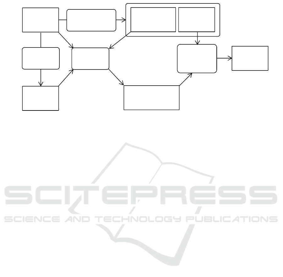
Figure 3: Process pipeline of the system.

4 EVALUATION

In this section, we describe the actual application of

our attribute influence scoring method to the digital

marketing use case to evaluate its validity. In this use

case, it treats huge number of customer data stored in

the CRM system. The attributes of customer

information includes customers’ service related

information such as member rank, number of system

to the fundamental personal information such as

address, age, sex and so on. The target model is the

deep learning model to predict the member rank in the

next year from the customer’s information. We

actually generate the model with CRM data and apply

our method to analyze the model and customer data.

4.1 Global Tendency Analysis based on

Target Data Segment

In the customer data used in our evaluation, there is

the member rank attribute in it. Member rank has 7

grades from 0 to 6 where rank 0 is free member and

other rank member is paid member. If the number of

rank is bigger, the customer is higher premium member.

The objective to implement measures on the marketing

is to make the member’s rank be higher and understand

the characteristics of members in each rank.

Because objective of this analysis is considera-

tion of methods for member to be higher rank, we

focus on the deep learning model for rank up

prediction as the analysis target. Input of this model

is member’s information and its output is probability

to be which rank in the next year. At first, we divide

customers’ data. In this case, we would like to analyze

rank up factor. So we divide data into 7 classes based

on the current rank. In the next step, self-organizing

maps are generated for all divided datasets. Then, we

applied LIME to each node on the map to calculate

the attribute influence score map. Because calculated

score map indicates stochastic increase for each

attribute and predicted rank, we can obtain rank up

score for each attribute by adding score maps as for

rank up of membership. Furthermore, it is also

possible to calculate the global tendency score by

taking weighted average using hitmap. Table 1

describes the top 3 list of influential attributes to

increase the member rank in each current rank. The

absolute value of the score indicates the influential

degree of the attribute. Items in the table are listed

descending order of the absolute value of the score.

Here, the attribute name written in the form of

“attribute = value” represents a category attribute. In

this case, the score indicates the increment rate of the

classification probability from current rank to upper

rank when the category attribute value changes to the

specific value. Other attributes such as total price of

purchased services take continuous value. In that

case, the score indicates the increase rate of classifica-

tion probability to upper rank when the input attribute

value increases for the size of standard deviation.

In terms of the overall tendency of the score, the

absolute value of the score contributing to the rank up

is smaller as the current rank is higher. Conversely,

this result can also conclude that the higher the rank

of member is, the lower the risk of ranking down is.

From current rank 0 to 2, attributes related to

automatic continuation of membership, elapsed days

from last purchase, and member card application

appear in the top 3, whereas as the ranking becomes

Learning

data

2. Generate self-

organizing map

Self-organizing

map

Model

Attribute influence

score map

1. Generate

model

3. Apply

LIME

Hitmap

4. Calculate

weighted

average

Total

score

A Causality Analysis for Nonlinear Classiﬁcation Model with Self-Organizing Map and Locally Approximation to Linear Model

423

Table 1: Globally calculated influence score of input attribute.

Current

Rank

Large influential attributes

1st 2nd 3rd

0 Automatic continuation of membership

0.387

Elapsed days from last purchase

-0.124

Member card application

0.109

1 Automatic continuation of membership

0.511

Elapsed days from last purchase

-0.197

Member card application

0.138

2 Automatic continuation of membership

0.365

Elapsed days from last purchase

-0.179

Member card application

0.110

3 Automatic continuation of membership

0.114

Elapsed days from last purchase

-0.091

Total price of purchased services

0.077

4 Total price of purchased services

0.033

Initial rank=3

-0.025

Initial rank=5

0.021

5 Total price of purchased services

0.034

Initial rank=3

-0.028

Number of purchased services

-0.025

6 Total price of purchased services

0.022

Number of purchased services

0.024

Number of purchased services

-0.20

higher, attributes relating to expenditure such as total

price of purchased services and initial member rank

are emphasized. These calculated trends are easy to

understand and make sense for humans. Furthermore,

while the total price of purchased services contributes

positively to the rank from 3 to 6, the sign of score for

number of purchased services is negative when the

current rank is 5 or higher (the score of the frequency

number of service purchase at rank 5 is -0.025). From

this result, it can be seen that purchase of the service

with the higher unit price is more important than the

number of service purchases in order for the premium

members to increase the member rank further more.

At current rank 3 or less, not only the automatic

continuation of membership but also the elapsed days

from the last service purchase are strongly related to

the rank up of membership. Since the sign of the

attribute of elapsed days is negative, the possibility of

rank decreases as the number of elapsed days

increases. From this result, it is understood that

regular following up measures for purchasing

services are important, particularly for members who

are in lower rank. Using the global tendency score of

attribute influence degree for each target rank of

customers, useful information on the direction of the

rank-up measures for each layer can be obtained as

described above.

4.2 Visualization of Predicted Rank

and Attribute Score

In this section, we analyze the trend of the attribute

influence degree obtained from the global tendency

score in more detail. From the result in the previous

section, we can say that the influence degree of the

automatic continuation of membership attribute is

larger at lower rank from 0 to 3. Figure 4 shows an

example of attribute influence score maps and

component maps on automatic continuation of

member attribute for current rank 0 and 3. The

component map is the self-organizing map generated

from the target data and score map is generated from

the LIME score for each node on the component map.

The global tendency score discussed in the previous

section is the sum of the all scores for rank up from

the current rank. Here we focus on the score maps for

individual rank prediction from the target current rank

to analyze our use case in more detail. Actually,

looking at them, it is possible to grasp which nodes or

clusters are affected strongly to predict higher rank in

terms of the analyzing attribute.

Score maps in (b) of the figure show the distributions

of LIME score for current rank 3 predicted to rank 3

to 5 individually. If we consider the rank up from

current rank 3, we should check out the score map of

prediction rank 4 or higher. In these score maps, since

the green node indicates that its score is 0, it is

possible to easily search for the node with red or blue

color on which the influence degree appears greatly.

Also, (c) of the figure shows the component maps of

the automatic continuation of membership attribute.

From these maps, it can be seen that the automatic

continuation of membership flag is not substantially

set for any customer in the case of current rank 0,

whereas customers who set automatic continuation

flag in the service site are biased to the left part of the

map in the case of current rank 3. Comparing this

component map with the score map of predicted rank

4 in (b), we can see that the red part on the score map

is similar to the relatively low blue part on the

component map. From this fact, it can be confirmed

that there is a possibility of low blue part on the

component map. From this fact, it can be confirmed

that there is a possibility of effectively working for

members in the blue part who are not set to automatic

continuation configuration when executing measures

related to the promotion of automatic continuation of

membership configuration.

ICAART 2019 - 11th International Conference on Agents and Artiﬁcial Intelligence

424

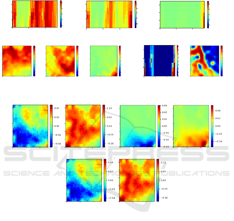
(a) Score map for current rank 0 on automatic continuation attribute.

(b) Score map for current rank 3 on automatic continuation

attribute.

Figure 4: Score map and component map on the attribute for automatic continuation of membership.

(a) Score map for current rank 3 and predicted rank 4. (b) Score map for current rank 3 and predicted rank 5.

Figure 5: Score map and component map on total price of purchased services.

Figure 5 shows score maps and component maps

for attributes of the total number of purchased

services and the total price of purchased services at

current rank 3. In the description on the global

tendency score analysis in the previous section, the

score for the number of purchased services is negative

in the current rank 3 or higher. As you can see on the

left map in Figure 4 (a), the score is positive in the

upper right, the lower right, and the middle three

places. This means the negative influence is not

uniform on the whole nodes even if the global

tendency score is negative. On the other hand, the

portion where the influence degree of both attributes

is larger with respect to the prediction rank 5 in (b) is

similar to the shape of larger value portion in the

component map of (c). From this fact, it is considered

that measures in terms of service purchase need to be

individually implemented for each member’s feature

represented by reference vectors of these nodes on the

map. However, the visualized component maps of

data with multiple attributes often become complex

patterns because of the complex data structure. It is

necessary to consider the method of grasping

customers represented by nodes.

From the above analysis, it can evaluate the

detailed influence degree for each node by grasping

the attribute with high influence degree at each target

rank by the global tendency score and visualizing the

score for each prediction class and attribute using the

self-organizing map. Applying the proposed method,

Predicted rank 4

Predicted rank 5

-0.05

-0.10

0.00

0.05

0.10

Predicted rank 3

-0.20

0.00

0.20

0.40

-0.40

-0.02

-0.04

0.00

0.02

0.04

Predicted rank 3

Current rank 0

Current rank 3

Predicted rank 4

Predicted rank 5

-0.20

0.00

0.20

0.40

-0.40

0.00

0.10

0.20

-0.20

-0.10

0.00

0.04

0.08

-0.04

-0.08

0.00

0.04

0.08

0.12

0.16

0.20

0.40

0.60

0.80

A Causality Analysis for Nonlinear Classiﬁcation Model with Self-Organizing Map and Locally Approximation to Linear Model

425

it is possible to provide useful information that can be

utilized for planning customers' measures for

membership rank up.

5 CONCLUSIONS

In this paper, we proposed the attribute influence

scoring method to address the relationship among

input and output data of the nonlinear classification

model with self-organizing map and locally

approximation to linear models. The proposed

method clarifies local characteristic with LIME score

on each node on the constructed self-organizing map.

It also shows global attribute influence score by

calculating weighted average value with LIME score

and hit count on every node. Thus, our method

enables analysts to have object-wise, cluster-wise and

global views in terms of targeting nonlinear model.

We applied our method to the actual use case of

customers’ membership rank-up analysis for digital

marketing to evaluate the validity of our method.

REFERENCES

Cai, Z., Fan, O., Feris, R., Vasconcelos, N., 2016. A unified

multiscale deep convolutional neural network for fast

object detection. In Proceedings of the 14

European

Conference on Computer Vision.

Agarwal, S., Awan, A., Roth, D., 2004. Learning to detect

objects in images via sparse, part-based representation.

In IEEE transactions on pattern analysis and machine

intelligence, 26, 11.

Hannun, A., Case, C., Casper, J., Catanzaro, B., Diamos, G.,

Elsen, E., Prenger, R., Satheesh, S., Sengupta, S.,

Coates, A., Ng, A., 2014. Deep Speech: Scaling up end-

to-end speech recognition. In arXiv:1412.5567.

Hannun, A., Maas, A., Jurafsky, D., and Ng, A., 2014. First-

Pass Large Vocabulary Continuous Speech Recognition

using Bi-Directional Recurrent DNNs. In arXiv:1408.

2873.

Ribeiro, M., Singh, S., and Guestrin, C., 2016. Why Should

I Trust You?: Explaining the Predictions of Any

Classifier. In Proceedings of NAACL-HLT 2016.

Le, Q., Ranzato, M., Monga, R., Devin, M., Chen, K.,

Corrado, G., Dean, J., and Ng, A., 2012. Building High-

level Features Using Large Scale Unsupervised

Learning. In Proceedings of the 29

International

Conference on Machine Learning.

Mahendran, A. and Vedaldi, A., 2014. Understanding Deep

Image Representations by Inverting Them. In arXiv:

1412.0035.

Smilkov, D., Thorat, N., Kim, B., Viegas, F., and

Wattenberg, M., 2017. SmoothGrad: removing noise by

adding noise. In arXiv: 1706.03825.

Springenberg, J., Dosovitskiy, A., Brox, T., and Riedmiller,

M., 2015. Striving for Simplicity: The All

Convolutional Net. In Proceedings of ICLR-2015.

Koh, P. and Liang, P., 2017. Understanding Black-box

Predictions via Influence Functions. In Proceedings of

the 34

International Conference on Machine

Learning.

Tolomei, G., Silvestri, F., Haines, A., and Lalmas, M., 2017.

Interpretable Predictions of Tree-based Ensembles via

Actionable Feature Tweaking. In KDD-2017.

Selvaraju, R., Cogswell, M., Das, A., Vedantam, R., Parikh,

D., Batra, D., 2017. Grad-CAM: Visual Explanations

from Deep Networks via Gradient-based Localization.

In arXiv: 1610.02391v3.

ICAART 2019 - 11th International Conference on Agents and Artiﬁcial Intelligence

426