Unscented Model Predictive Control (UMPC) for Ship Heading
Control with Stochastic Disturbance
Baity Jannaty
1,a
, Subchan, and Tahiyatul Asfihani
1
Department of Mathematics, Institut Teknologi Sepuluh Nopember, Indonesia
Keywords: Model Predictive Control, Ship Heading Control, Stochastic Disturbance, Unscented Kalman Filter.
Abstract: This paper discussed a ship heading control problem with Unscented Model Predictive Control (UMPC).
Rudder angle is controlled such that the heading angle follows the desired angle. This paper used model with
three degrees of freedom, that is sway, yaw, and roll. UMPC is based on Model Predictive Control (MPC) for
nonlinear system with stochastic disturbance. There are noises in the system model, therefore the system
become dynamic stochastic with probabilistic constraint. These noises cause a changing in the state variable
from a definite value to a distributed random variable. The objective function change from deterministic into
the form of expectations of random variable. state variable constraints are changed from probabilistic to
deterministic to address this issue. The objective function is changed into deterministic forms. System is
linearized using stochastic linearization to approximate state transition. The Unscented Kalman Filter (UKF)
is used as prediction process for MPC. The prediction process result is used by MPC algorithm by minimizing
the objective function. The computation results showed that UMPC can handle problem with stochastic
disturbance.
1 INTRODUCTION
Ship heading is one of the control problems in the
marine field which have attracted great attention of
researchers (Li and Sun, 2012, Fossen, 1994). A Ship
requires a navigation system, guide, and control that
is able to direct it to the desired angle (Perez, 2005,
and Subchan and Zbikowski, 2009). One of the
popular control method that have been applied in
industry is Model Predictive Control (MPC) (Qin and
Badgwell, 2003). MPC has some advantages
compared to other controllers, such as the ability to
predict the future process outputs, without ignoring
the constraints (Bordons and Camacho, 2007, and
Holkar 2010). MPC can also able to control wide
range of process ranging from systems with relatively
simple dynamics to systems with higher complexity,
including system with long delay or unstable systems
(Yoon, 2007 and Liuping, 2009).
Some works have been done to control the
heading angle using MPC, using one degree of
freedom (Subchan, 2014; Naveen, 2014), two degrees
(Subchan, 2014), three degrees (Wang, 2010), and
four degrees of freedom (Cahyaningtyas, 2014). In
the previous studies, MPC is only able to control
systems with measurable disturbance. In fact, the
model’s uncertainty of the model and stochastic
disturbance are natural characteristic of the system
model (Li, 2000, and Syafii, 2019).
Unscented Model Predictive Control (UMPC) is
MPC for non-linear systems that can handle
probabilistic constraints with approximating
uncertainty in the model (Farrokhsiar, 2012). The
Unscented Kalman Filter replaces the prediction
process in MPC. System is linearized using stochastic
linearization to approximate state transition (Wan and
Merwe, 2000). In this work, UMPC is used to control
the heading angle of non-linear stochastic system
with three degrees of freedom.
2 LIFTING EQUIPMENT
This section explains the specifications of ship,
mathematical model, and unscented model predictive
control method.
2.1 Specification of Ship
The specification of ship is given in Table 1.
Jannaty, B., Subchan, . and Asfihani, T.
Unscented Model Predictive Control (UMPC) for Ship Heading Control with Stochastic Disturbance.
DOI: 10.5220/0010854200003261
In Proceedings of the 4th International Conference on Marine Technology (senta 2019) - Transforming Maritime Technology for Fair and Sustainable Development in the Era of Industrial
Revolution 4.0, pages 97-103
ISBN: 978-989-758-557-9; ISSN: 2795-4579
Copyright
c
 2022 by SCITEPRESS – Science and Technology Publications, Lda. All rights reserved
97

Table 1: Ship specification.
Quantity (Symbol) Value (Unit)
Length ( 𝐿
𝑝𝑝
)
48 (meter)
Width ( 𝐵 )
8.6 (meter)
Draft ( 𝐷 )
2.2 (meter)
Mass ( 𝑚 )
359 × 10
3
(kg)
Volume of displacement (∇)
350 (mete
r
3
)
Yaw Inertia (𝐼
𝑧
)
33.7 × 10
6
(kg meter
2
)
Roll Inertia (𝐼
𝑥
)
3.4 × 10
6
(kg meter
2
)
Coordinate cente
r
of gravitation (𝑥
𝐺
)
-3.38 (meter)
Coordinate cente
r
of gravitation (𝑧
𝐺
)
-1.75 (meter)
Rudder area ( 𝐴
𝑅
)
0.73 (meter)
Coefficient of lift force (𝐶
𝐿
)
1.15
Distance CG-CP (𝐼
𝛿𝑧
)
1.2 (meter)
LCG (𝑙
𝛿𝑧
)
-23.5 (meter)
Metacenter (𝐺𝑍)
0.776 (meter)
Density of water (𝜌)
9.82 (meter/s
2
)
2.2 Ship Dynamical Model
The kinematic model of ship as follows:
𝜙  𝑝
1
𝜓  𝑟𝑐𝑜𝑠 𝜙
2
Where 𝑝, 𝑟, 𝜓, 𝜙 denote respectively roll rate, yaw
rate, yaw angle and roll angle in inertial form.
The purpose of control is to control the rudder
angle (𝛿) therefore the value of yaw angle as desired.
Using kinematic model in Equation (1) and (2), and
ship mathematical model with four degrees of
freedom (Fossen, 1998), with assumption that surge
velocity is constant, general dynamical model of ship
with three degrees of freedom is shown below:
⎣
⎢
⎢
⎢
⎡
v

p

r
ϕ

φ ⎦
⎥
⎥
⎥
⎤

⎣
⎢
⎢
⎢
⎡
a

b

c

0
0
a

b

0
0
0
a

0
c

0
0
0
0
0
1
0
0
0
0
0
1
⎦
⎥
⎥
⎥
⎤

⎩
⎪
⎨
⎪
⎧
⎣
⎢
⎢
⎢
⎡
mUr Y

mz

UrK

mx

Ur N

0
0
⎦
⎥
⎥
⎥
⎤

⎣
⎢
⎢
⎢
⎡
Y


K


N


0
0
⎦
⎥
⎥
⎥
⎤
δ

⎭
⎪
⎬
⎪
⎫
3
Where:
𝑎
1
 𝑚  𝑌𝑣
𝑎
2
 𝑚𝑧𝐺  𝑌𝑝
𝑎
3
 𝑚𝑥𝐺  𝑌𝑟
𝑏
1
 𝑚𝑧𝐺  𝐾𝑣 , 𝑏
2
 𝐼𝑧  𝐾𝑝
𝑐
1
 𝑚𝑥𝐺  𝑁𝑣 , 𝑐
2
 𝐼𝑧  𝑁𝑟
Equation (3) discretized using forward difference
method with Δ𝑡 = 0.1. From Equation (3), define state
space of model as below:
𝑥 = [𝑣, 𝑝, 𝑟, 𝜙, 𝜓] 4
Model in Equation (3) can be written as follow:
𝑥 
𝑓
𝑥, 𝑢 5
𝑦 𝑔𝑥, 𝑢 6
Equation (5) stated mathematical model, with 𝑢 is
input system, that is rudder angle. While Equation (6)
define output of model, in this case is yaw angle.
Equation (5) and (6) is standard model system where
there is no noise inherent in the system model. In the
real, the presence of noise cannot be ignored.
Therefore, system model can be defined as follow:
𝑥̇ =
𝑓
(𝑥, 𝑢) + 𝑤𝑘 5
𝑦 = 𝑔(𝑥, 𝑢) + 𝑣𝑘 6
Where 𝑤𝑘~𝑁 (0, 𝜏), that is normal distribution with
mean 0 and variance 𝜏 and 𝑣𝑘~𝑁(0, Λ), that is normal
distribution with mean 0 and variance Λ.
The presence of noise causes system changes
from deterministic to stochastic. MPC standard
cannot be applied, therefore in the next section is
formulated Unscented Model Predictive Control
method to control system in Equation (5) and (6).
3 FORMULATION UNSCENTED
MODEL PREDICTIVE
CONTROL
Unscented Model Predictive Control method
(UMPC) is stochastic MPC for non linear systems
that approximates the transition from state variable
using unscented transformation as statistic
linearization method (Bradford, 2017). With
assumption that control horizon equal to the
prediction horizon (𝑁
𝑐
= 𝑁
𝑝
), the objective function
defined as follow:
min
𝑢
𝐽



𝑦

𝑘𝑖|𝑘

𝑦



𝑄

𝑦

𝑘



𝑖 |𝑘

𝑦


𝑢

𝑘𝑖1 | 𝑘


𝑅𝑢

𝑘
𝑖1| 𝑘



(7)
senta 2019 - The International Conference on Marine Technology (SENTA)
98

With constraints:
𝑥𝑘+1 =
𝑓
(𝑥𝑘, 𝑢𝑘, 𝑘) 8
𝑥𝑚𝑖𝑛 ≤ 𝑥(𝑘 +
𝑗
∣ 𝑘) ≤ 𝑥𝑚𝑎𝑥 9
𝑢𝑚𝑖𝑛 ≤ 𝑢 (𝑘 +
𝑗
− 1 ∣ 𝑘) ≤ 𝑢𝑚𝑎𝑥 10
Formulation Unscented Model Predictive Control
(UMPC) is described below:
3.1 The Application of Unscented
Kalman Filter (UKF) for the
Prediction Process on MPC
The optimization problem solved in this research is in
the form of dynamics stochastic, which the values of
state variables represented by a distributed random
variable. This condition prevents the MPC method
from not being used. In this research, Unscented
Kalman Filter (UKF) was used to replace the
prediction process on MPC (Changchun, 2014). The
UKF in the case of additive noise for (5) and (6) to
approximate mean and covariance can be stated as
follows (Subchan, 2019).
1. Definition of Sigma-points
𝜒
𝑘  𝑗  1 ∣ 𝑘  𝑥̂ 𝑘  𝑗  1 ∣ 𝑘
𝑥̂ 𝑘  𝑗  1 ∣ 𝑘 
√
𝐿  𝜆 𝑃1⁄2𝑘  𝑗  1 ∣ 𝑘
𝑥̂

𝑘  𝑗  1 ∣ 𝑘


√
𝐿  𝜆 𝑃1⁄2

𝑘  𝑗  1 ∣ 𝑘

11
2. Covariance and mean approximation of
predictions
𝑋





𝑓
𝑥



,𝑢


(12)
𝑋


 𝑊




𝑋









(13)
𝑃

  𝑊




𝑋






𝑋


𝑋




𝑋




𝑀


(14)
3. Covariance and mean approximation of
observations:
𝑌




𝑔𝑋


(15)
𝑦

𝑊




𝑌









(16)
𝑆

 𝑊





𝑌







 𝑦


𝑌




𝑋




𝐶𝑜𝑣

(17)
𝑃

,
𝑊







𝑋




𝑋



𝑌





𝑦




(18)
𝐾

𝑃

,
𝑆


(19)
𝑋


𝑋


(20)
𝑃

𝑃


𝐾

𝑆

𝐾


(21)
3.2 Changing State Variable
Constraint from Probabilistic to
Deterministic
Objective function and constraints are defined in
Equation (7)-(10) in deterministic form. The
existence of noises causes a shift in the state variable
from a definite value to a distributed random variable.
The objective function change from deterministic into
the form of random quantity expectations. The
stochastic dynamic optimization problem can be
written below.
min
𝑢
𝐽
𝐸


𝑦

𝑘1|𝑘

𝑦



𝑄

𝑦

𝑘



𝑖|𝑘

𝑦


𝑢

𝑘𝑖1|𝑘


𝑅𝑢

𝑘
𝑖1|𝑘


(22)
With constrains:
𝑥


𝑓

𝑥

,𝑢


𝑤

(23)
𝑦

𝑔

𝑥

,𝑢


𝑣

(24)
𝑃

𝑥


𝛽


𝑝


,𝑖1,…,𝑛,
𝑗
1,…,𝑁

(25)
𝑢

𝜇

,
𝑗
0,…,𝑁

1
(26)
Where 𝑥
𝑖
stated in the I th element from state variable
𝑥
k+j,
𝛽


is state variable constraints, while β is
probability of state constraints.
Input constraint in Equation (26) still in the form
deterministic because its value not affected by state
variable. State constraints in Equation (25) be
changed in the form of deterministic. Suppose 𝑥̂𝑘
+
𝑗
+1
,
mean value from random variable, where
𝑘
+
𝑗
+1
∼, 𝑁(0,
𝑃
𝑘
+
𝑗∣𝑘
), that is normal distribution with mean 0 and
variance 𝑃
𝑘
+
𝑗∣𝑘
. Given 𝜉
𝑘
+
𝑗
= 𝑃1/2 𝑥̂𝑘+𝑗∣𝑘 has
Unscented Model Predictive Control (UMPC) for Ship Heading Control with Stochastic Disturbance
99

standard normal distribution N (0,1), Then,
𝑃

𝑥

𝛽

𝑝

𝑃𝜀

𝛽


𝑝

where
𝛽








|


/
. Suppose 𝛽


∗
solution from 𝜗𝛽


∗

𝑝

, with 𝜗. is the standard normal distribution
function (Sahoo,2013). Then constrain in Equation
(25) can be recast as:
𝑥
|
𝛽

𝑃
|


𝛽

∗

(27)
Constraint in Equation (27) have been in the form
of deterministic.
3.3 Changing Objective Function from
Random Quantity Expectation to
Deterministic
Objective function that defined in Equation (22) is in
the form of random quantity expectation. Based on
probability theory, objective function in Equation
(22) can be changed as follow.
𝐽
𝑡𝑟

𝐸

𝑦𝑦


𝑦𝑦




𝑄

𝑢

𝑅𝑢





(28)
Yan and Bitmead, 1990, showed that solving the
stated in Equation (28) is equivalent to solving a
deterministic dynamic programming:
min
𝑢
𝐽


𝑦

𝑘𝑖|𝑘

𝑦



𝑄

𝑦

𝑘



𝑖|𝑘

𝑦


𝑢

𝑘𝑖1|𝑘


𝑅𝑢

𝑘
𝑖1|𝑘



(29)
Subject to Equation (11)-(21) and (26)-(27). In the
next section, numerical evaluations of the Equation
(29) are discussed.
4 SIMULATIONS
In this section, the simulation results are displayed
followed by a discussion of the systems performance
analysis. The purpose of control in this research is to
control the rudder angle (𝛿) therefore the value of yaw
angle (𝑦) as expected (𝑦𝑑) with minimum energy (𝑢).
In simulation is used a discrete system with discretion
time Δ𝑡 = 0.1. Given constraint in rudder angle and
yaw velocity respectively |𝛿| ≤ 35° and |𝑟| ≤ 0.0932
𝑟𝑎𝑑/𝑠. Total time for simulation are 300 seconds. The
weighting matrix 𝑄 = 200, 𝑅 = 10, with noise 𝑤𝑘
∼ 𝑁(0,10−4) and 𝑣𝑘 ∼𝑁(0,10−2). Initial value of
state variable described as follow.
𝑥
0
= [0 0 0.0853 𝑟𝑎𝑑/𝑠 0 30°]
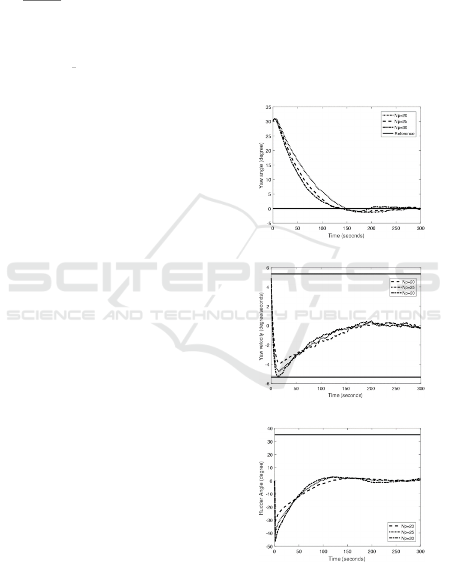
30
In the first simulation was simulated UMPC with
different value of prediction horizon, that is 𝑁𝑝 =
20,25, and 30. Figure 1 shows that the heading angle
can reach the desired heading angle, that is 0°. From
Figure 2 and Figure 3, the yaw rate and rudder angle
satisfy the given constraints.
Figure 1: Yaw angle with UMPC method.
Figure 2: Yaw velocity with UMPC method.
Figure 3: Rudder angle with UMPC method.
senta 2019 - The International Conference on Marine Technology (SENTA)
100

Then the comparison of the RMSE for each
prediction horizon is considered. The following
equation is used to compute the RMSE.
𝑅𝑀𝑆𝐸

∑
𝑦

 𝑦



 

𝑇𝑜𝑡𝑎𝑙 𝑡𝑖𝑚𝑒
31
Where 𝑦
𝑖
and 𝑦
𝑑𝑖
are the heading angle at time 𝑖 and
the desired heading angle at time 𝑖.
Table 2: Comparison of the RMSE for each prediction
horizon.
Prediction Horizon (𝑁
𝑝
)
RMSE
20 11.7418023
25 10.3627875
30 9.3963874
According to Table 2, the smallest RMSE is reached
when 𝑁𝑝 = 30. In the next simulation is used 𝑁𝑝 =
30.
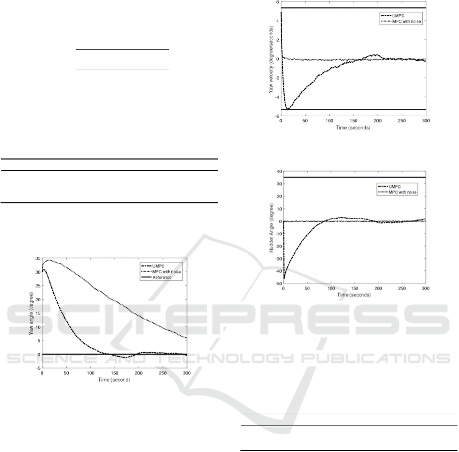
Figure 4: Comparison yaw angle between UMPC and MPC
with noise.
The second simulation will compare performance
system between UMPC and MPC with noise. In the
simulation using MPC with noise, stochastic model
system with deterministic constraints is simulated.
Figure 4 shows in the end of the simulation, heading
angle when controlled using MPC with noise has not
reached the reference yet. But using UMPC, it
reaches reference angle in time 148 seconds. From
Figure 5 and Figure 6, the yaw rate and rudder angle
satisfy the given constraints.
Figure 5: Comparison yaw velocity between UMPC and
MPC with noise.
Figure 6: Comparison rudder angle between UMPC and
MPC with noise.
The third simulation is carried out by varying the
noise values. The scenarios is given in Table 3, where
𝑤
𝑘
is noise in the system model and 𝑣
𝑘
is noise in the
measurement model.
Table 3: Noise variations for simulation using UMPC.
Scenario
𝑤
𝑘
𝑣
𝑘
1
𝑁(0,10
−4
) 𝑁(0,10
−2
)
2
𝑁(0,10
−2
) 𝑁(0,10
−2
)
In Figure 7, heading angle in Scenario 1 can
reached the reference point faster than Scenario 2. In
The yaw angle in Scenario 1 reaches the reference at
148 seconds. While in Scenario 2, the yaw angle
reaches the reference at 390 seconds. A large noise
value of system model in Scenario 2 causes the
additional time which needed to reach the reference.
From Figure 8 and Figure 9, the yaw rate and rudder
angle satisfy the given constraints.
Unscented Model Predictive Control (UMPC) for Ship Heading Control with Stochastic Disturbance
101

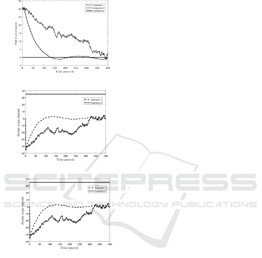
Figure 8: Comparison yaw velocity.
Figure 9: Comparison rudder angle.
5 CONCLUSIONS
In this paper Unscented Model Predictive Control
(UMPC) used to solve the ship heading control
problem. This approach uses the Unscented Kalman
Filter (UKF) to replace prediction process in MPC.
UMPC can handle problem with stochastic
disturbance. The simulation results show that the
whole constraints are satisfied with variation in noise
value and prediction horizon. In this work, the
weighting matrices are 𝑄 = 200 and 𝑅 = 10. From
simulation, best performance reached with 𝑁𝑝 = 30.
ACKNOWLEDGEMENT
This work was supported by DPRM RISTEKDIKTI
contract number 895/PKS/ITS/2019 and Institut
Teknologi Sepuluh Nopember contract number
1192/PKS/ITS/2019.
REFERENCES
Bradford, Eric, and Imsland, L., 2017. Stochastic Nonlinear
Model Predictive Control with State Estimation by
Incorporation of the Unscented Kalman Filter.
Bordons, C., and Camacho,E.F., 2007. Model predictive
control, Springer. London.
Changchun, L., Andrew, G., Chankyu, L., Hedrick, J.K.,
Pan, J., 2014. Nonlinear stochastic predictive control
with unscented transformation for semi-autonomous
vehicles, 2014 American Control Conference (ACC)
June 4-6, 2014. Portland, Oregon, USA.
Wan, E., and Merwe, R.V., 2000. The unscented kalman
filter for nonlinear estimation, in Adaptive Systems for
Signal Processing, Communications, and Control
Symposium 2000. AS-SPCC. The IEEE2000, pp. 153-
158.
Wang, Z., Zou, Y., and Li, 2010. Path following control of
underactuated ships based on unscented kalman filter,
Journal of Shanghai Jiaotong University (Science), Vol.
15, No.1, pp.108-113.
Fossen, T.I., 1994. Guidance and control of ocean vehicles,
Hoboken: Wiley.
Holkar, 2010. An overview of model predictive control,
International Journal of Control and Automation, Vol.3,
No.4.
Syafii, A.M., 2019. Kendali haluan kapal dengan
menggunakan modifikasi Model Predictive Control-
Kalman Filter, Master thesis: Institut Teknologi
Sepuluh Nopember.
Yoon, H.K., Son, N.S., and Lee, G.J., 2007. Estimation of
the roll hydrodynamic moment model of a ship by using
the system identication method and the free running
model test, Maritime and Engineering Reaseach
Institute. Korea, Daejon 305-600.
Li, P., Wendt, M., and Wozny, G., 2000. Robust model
predictive control under chance constraints, Computers
and Chemical Engineering 24: 829-834.
Li, Z. and Sun, J., 2012. Disturbance compensating model
predictive control with application to ship heading
control, IEEE Vol.20 No.1.
Liuping, W., 2009. Model predictive control system design
and implementation using MATLAB, Springer.
London. Farrokhsiar, M. and Najjaran, H., 2012. An
unscented model predictive control approach to the
formation control of nonholonomic mobile robots,
IEEE International Conference on Robotics and
Automation
River Centre. Saint Paul, Minnesota, USA.
Figure 7: Comparison yaw angle.
senta 2019 - The International Conference on Marine Technology (SENTA)
102

Perez, T., 2005. Ship Motion Control: Course Keeping and
Roll Stabilization using Rudder and Fins, Advances in
Industrial Control.
Qin, J. and Badgwell, T., 2003. An overview of industrial
model predictive control technology, Department of
Chemical Engineering, Rice University. Houston,
TX77251.
Julier, S.J., Uhlmann, J.K., and Durrant, W.H., 1995. A new
approach for filtering nonlinear systems, in Proceedings
of the American Control Conference, pp. 1628-1632.
Julier, S.J. and Uhlmann, J.K., 1997. A new extension of
the kalman filter to nonlinear systems, in Proceedings
of Aero Sense: The 11th International Symposium on
Aerospace Defence Sensing, Simulation and Controls.
Cahyaningtyas, S., 2014. Penerapan Disturbance
Compensating Model Predictive Control (DC-MPC)
Pada Kendali Gerak Kapal, Jurnal Sains dan Seni,
hal:1-7.
Sahoo, P., 2013, Probability and Mathematical Statistics,
University of Louisville, Louisville.
Subchan, S., 2008. A direct multiple shooting for the
optimal trajectory of missile guidance, In: 2008 IEEE
. International Conference on Control Applications
IEEE, p.268-273
Subchan S. and Zbikowski, R, 2007 Computational optimal
control of the terminal bunt manoeuvre—Part 1:
minimum altitude case, Optim. Control Appl. Meth.,
28: 311-353. doi:10.1002/oca.807
Subchan, S. and Żbikowski, R., 2007, Computational
optimal control of the terminal bunt manoeuvre—Part
2: minimum‐time case. Optim. Control Appl. Meth.,
28: 355-379. doi:10.1002/oca.806
Subchan, Syaifuddin, W.H., dan Asfihani, T., 2014. Ship
heading control of corvette-sigma with disturbances
using model predictive control, Far East Journal of
Applied Mathematics vol. 87, No.3, pp.245-256.
Subchan, Ismail, R.W., and Asfihani, T., 2019. Estimation
of Hydrodynamic Coefficients Using Unscented
Kalman Filter and Recursive Least Square, IEEE 11th
International Workshop on Computational Intelligence
and Applications.
Yan, J. and Bitmead, R.R., Incorporating state estimation
into model predictive control and its application to
network traffic control, Automatica 41:595-604.
Zhu, Y. and Ozguner, U., Constrained model predictive
control for nonholonomic vehicle regulation problem,
in Proceedings of the 17th IFAC World Congress, pp.
9552-9557.
Zheng, H. and Negenborn, R.R., 2014. Trajectory tracking
of autonomous vessels using model predictive control,
The International Federation of Automatic Control.
Unscented Model Predictive Control (UMPC) for Ship Heading Control with Stochastic Disturbance
103