
Stability Analysis of the SIRS Epidemic Model using
the Fifth-order Runge Kutta Method
Tulus
1
, T. J. Marpaung
1
, D. Destawandi
1
, J. L. Marpaung
1
and Suriati
2
1
Department of Mathematics, Universitas Sumatera Utara, Medan, Indonesia
2
Department of Informatics, Universitas Harapan Medan, Medan, Indonesia
Keywords: Runge-Kutta Method, SIRS Epidemic Model.
Abstract: Transmission of the disease occurs through interactions in the infection chain both directly and indirectly.
There are several causes of a disease that can enter endemic conditions, namely the condition of a disease
outbreak in an area for a long time. This condition can be modeled mathematically using certain assumptions
that will then be solved by analytical and numerical solutions. In this study, an analysis of the stability of
disease spread will be carried out by constructing a mathematical model of the SIRS epidemic in infectious
diseases. The results obtained are based on numerical solutions obtained through the Runge-Kutta 5th Order
Method. After that, analysis and simulation are done with the MATLAB program. In the simulation results,
it can be seen that the greater the rate of disease transmission or the low recovery rate and natural death causes
endemic conditions.
1 INTRODUCTION
The epidemic model studies the dynamics of the
spread or transmission of a disease in a population.
The SIRS epidemic model is an outgrowth of the SIR
epidemic model. The SIRS epidemic model differs
from the previous model when individuals who have
recovered can return to the susceptible class (Adda &
Bichara, 2012).
The numerical method is also called an alternative
to the analytic method, which is a method of solving
mathematical problems with standard or common
algebraic formulas. So, called, because sometimes
math problems are difficult to solve or even cannot be
solved analytically so it can be said that the
mathematical problem has no analytical solution.
Alternatively, the mathematical problem is solved by
numerical method, for which the Runge-Kutta
method of order 5 is used with a high degree of
accuracy (Xiaobin et al., 2018).
2 RUNGE-KUTTA ORDER 5
The fifth-order Runge-Kutta method is the most
meticulous method in terms of second, third and
fourth order (Sinuhaji, 2015). The fifth-order Runge-
Kutta order is derived and equates to the terms of the
taylor series for the value of n = 5 (Tulus, 2012).
The fifth-order Runge-Kutta can be done by
following the steps below:
𝑘
ℎ𝑓
𝑡
,𝑥
𝑘
ℎ𝑓
𝑡
,𝑥
𝑘
ℎ𝑓
𝑡
,𝑥
𝑘
ℎ𝑓
𝑡
,𝑥
𝑘
ℎ𝑓
𝑡
,𝑥
𝑘
ℎ𝑓
𝑡
ℎ,𝑥
𝑥
𝑥
1 / 90
7𝑘
32𝑘
12𝑘
32𝑘
7𝑘
3 MODEL FORMULATION
Let 𝑆
𝑡
,𝐼
𝑡
dan 𝑅
𝑡
successive states
subpopulation density of susceptible individuals is
infected and recovered, with number at time 𝑡
(Steven, 2017). In this model it is assumed that the
total population density at all times is constant, that is
(1)
376
Tulus, ., Marpaung, T., Destawandi, D., Marpaung, J. and Suriati, .
Stability Analysis of the SIRS Epidemic Model using the Fifth-order Runge Kutta Method.
DOI: 10.5220/0010187100002775
In Proceedings of the 1st International MIPAnet Conference on Science and Mathematics (IMC-SciMath 2019), pages 376-381
ISBN: 978-989-758-556-2
Copyright
c
2022 by SCITEPRESS – Science and Technology Publications, Lda. All rights reserved

𝑁𝑆
𝑡
𝐼
𝑡
𝑅𝑡. SIRS models discussed in
this paper compartment illustrated in the following
diagram:
Obtained system of ordinary differential
equations with three dependent variables were
respectively declared rate of change in density of
susceptible, infected and recovered:
𝛬
𝜇
𝑆𝛾𝑅
𝜇
𝛿𝛼
𝐼
𝛼𝐼
𝜇
𝛾
𝑅
Since the total population rate is equal to the rate
of death, then 𝛬 = 𝜇
𝑆
𝜇
𝛿
𝐼𝜇
𝑅, and 𝑆
𝐼𝑅𝑁 so the system becomes
𝜇
𝛿𝜇
𝛾
𝐼
𝜇
𝛾
𝑁
𝜇
𝛾
𝑆
𝜇
𝛿𝛼
𝐼
𝛼𝐼
𝜇
𝛾
𝑅.
If 𝑆
, 𝐼
and 𝑅
, then system (3.2) with
the first two equations can be simplified into:
𝛽𝑆𝐼
𝜇
𝛿𝜇
𝛾
𝐼
𝜇
𝛾
𝑆
𝜇
𝛾
𝛽𝑆𝐼
𝜇
𝛿𝛼
𝐼
𝛼𝐼
𝜇
𝛾
𝑅
Note that the first two equations in the system
(3.3) do not contain the variable R (t) so that for the
next reason enough to be discussed the system with
two equations. If the value of 𝑆
𝑡
and 𝐼
𝑡
has been
obtained, then the value of 𝑅𝑡 will be obtained by
using the relationship 𝑆𝐼𝑅𝑁.
4 RESULT
4.1 Disease Free Equilibrium Point
The equilibrium point is reached when the variable
that originally changes with time becomes constant.
Thus, the equilibrium point is obtained when
and
in equation (4) are zero.
𝛽𝑆𝐼
𝜇
𝛿𝜇
𝛾
𝐼
𝜇
𝛾
𝑆
𝜇
𝛾
0
𝛽𝑆𝐼
𝜇
𝛿𝛼
𝐼0
Based on equation (6) two possibilities are obtained,
namely 𝐼0 or 𝑆
. If 𝐼0 is substituted
in equation (5)
𝑑𝑆
𝑑𝑡
𝛽𝑆𝐼
𝜇
𝛿𝜇
𝛾
𝐼
𝜇
𝛾
𝑆
𝜇
𝛾
0
𝛽𝑆
0
𝜇
𝛿𝜇
𝛾
0
𝜇
𝛾
𝑆
𝜇
𝛾
0
𝜇
𝛾
𝑆
𝜇
𝛾
0
𝑆
𝜇
𝛾
𝜇
𝛾
1
obtained 𝑆1, so that obtained the disease-free
equilibrium point 𝐸
1,0.
4.2 The Endemic Equilibrium Point
The endemic equilibrium point is a point that
indicates the possibility of spreading the disease in
the population. In equation (6) if 𝑆
,
obtained equilibrium point is a second, which is the
point of equilibrium endemics 𝐸
∗
𝑆
∗
,𝐼
∗
, with
𝑆
∗
, then if the substitution of the equation
(5)
𝑑𝑠
𝑑𝑡
𝛽
𝜇
𝛿𝛼
𝛽
𝐼
∗
𝜇
𝛿𝜇
𝛾
𝐼
∗
𝜇
𝛾
𝜇
𝛾
0
is obtained 𝐼
∗
or 𝐼
∗
1
with 𝑅
is the basic
reproduction number. Note that the endemic
(2)
(3)
(4)
Stability Analysis of the SIRS Epidemic Model using the Fifth-order Runge Kutta Method
377

equilibrium point 𝐸
∗
𝑆
∗
,𝐼
∗
will exist when 𝑅
1.
4.3 Analysis of Local Stability on 𝑬
𝟎
The nature of local stability at equilibrium point E_0
is determined by linearizing the system of equation
(4) around the equilibrium point.
Suppose:
𝑓
𝑆,𝐼
𝛽𝑆𝐼
𝜇
𝛿𝜇
𝛾
𝐼
𝜇
𝛾
𝑆
𝜇
𝛾
𝑔
𝑆,𝐼
𝛽𝑆𝐼
𝜇
𝛿𝛼
𝐼
Then each function is derived partially to the
variable on the function, so that Jacobi matrix is
obtained
𝐽
𝑆,𝐼
𝛽𝐼
𝜇
𝛾
𝛽𝑆
𝜇
𝛿𝜇
𝛾
𝛽𝐼 𝛽𝑆
𝜇
𝛿𝛼
The system linearization of equation (4) around
the equilibrium point 𝐸
1,0
gives the Jacobi
matrix
𝐽
1,0
𝜇
𝛾
𝛽
𝜇
𝛿𝜇
𝛾
0𝛽
𝜇
𝛿𝛼
,
which has an eigen value 𝜆
𝜇
𝛾
0 and
𝜆
𝛽
𝜇
𝛿𝛼
or 𝜆
𝑅
1
𝜇
𝛿
𝛼
. If 𝑅
1 then 𝜆
0 so the equilibrium point 𝐸
is stable. Conversely, if 𝑅
1 then the equilibrium
point 𝐸
is unstable.
4.4 Analysis of Local Stability on 𝑬
∗
To obtain local stability properties in 𝐸
∗
, the
linearization around the endemic equilibrium point
𝐸
∗
𝑆
∗
,𝐼
∗
resulted in Jacobi matrix
𝐽
𝑆
∗
,𝐼
∗
𝜇
𝛿𝛼
𝑅
1
𝜇
𝛾
𝛼𝜇
𝛾
𝜇
𝛿𝛼
𝑅
1
0
.
obtained a complex eigen value 𝜆
,
𝑎𝑖𝑏, with
𝑎0. Therefore, the equilibrium point 𝐸
∗
is
asymptotically stable.
4.5 Model Solution with 5
th
Order
Runge-Kutta Method
Numerical analysis illustrates more clearly the model
of disease spread by using certain predefined
parameters and values. The system of equation (4)
will be solved by simulating the Runge-Kutta method
of order 5. The simulation of the SIRS epidemic
model solved by the 5th order runge-kutta method is
performed by giving the initial value of the
susceptible (𝑆, infected (𝐼, recovered (𝑅 individual
size, and varying the parameters that influence the
model interaction so that there will be 2 possibilities
that is 𝑅
1 and 𝑅
1. The initial values given
for the SIRS epidemic model for HSV disease are:
Table 1: The initial value of each subpopulation.
Subpopulation Initial value (million
souls)
𝑆
400
𝐼
200
𝑅
100
4.5.1 Simulation 𝑹
𝟎
1
For 𝑅
1, given the parameter values to qualify
𝑅
1, earned value 𝑅
0,6. The value of the
given value as follows:
Table 2: The parameter values R
1.
Paramete
r
Value
𝛼
0,013
𝛽
0,014
𝛾
0,007
𝛿
0,009
𝜇
0,001
𝜇
0,0013
𝜇
0,00115
From the initial value and the given parameter
values obtained simulation 𝑅
1 shown in Figure 1
& 2. Population 𝑆,𝐼,𝑅 experience changes with time,
indicating that the behavior of the solution will be
towards the point 𝐸
or it can be said that when 𝑅
1 the longer the epidemic disease will disappear from
the population.
Graphs do not reflect system behavior over time
ℎ0.09. So, it can be concluded at the time range
ℎ0.09 unstable system. The following is given a
table that describes the stability of the system depends
on the value of ℎ.
IMC-SciMath 2019 - The International MIPAnet Conference on Science and Mathematics (IMC-SciMath)
378
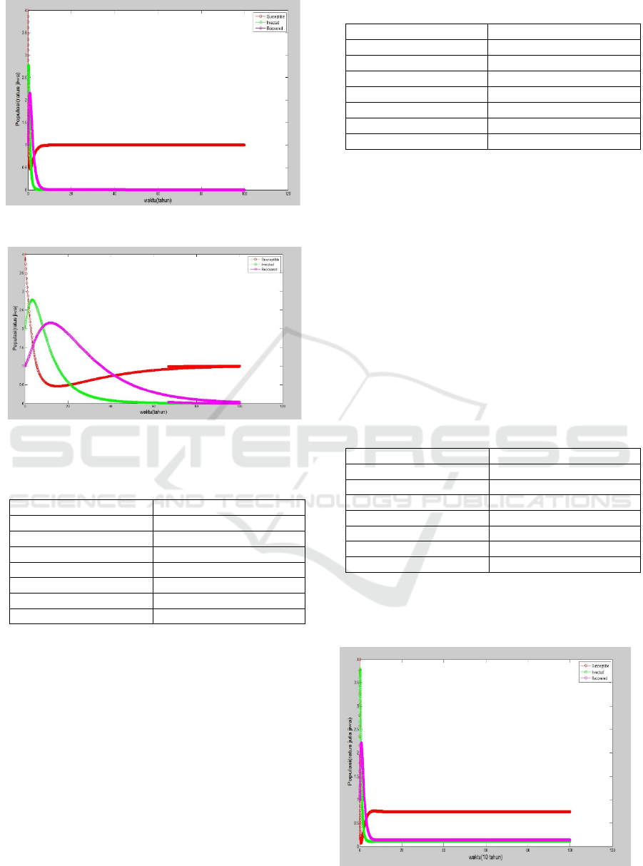
Figure 1: Simulation SIRS Model R
1 with h0.01.
Figure 2: Simulation SIRS Model R
1 with h0.09.
Table 3: The behavior of the system is based on the value
of h on the disease-free SIRS model.
Step time
ℎ
System behavior
0,01 Stable
0,02 Stable
0,03 Stable
0,05 Stable
0,07 Stable
0,08 Stable
0,09 Unstable
The graph does not show stability in the
population because ℎ is so large, the graph will be
stable if the ℎ value is less than 0,09.
4.5.2 Simulation 𝑹
𝟎
1
For 𝑅
1, given the parameter values to qualify
𝑅
1, from the values obtained value 𝑅
1,34.
The value of the given value as follows:
Table 4: The parameter values simulation 1 R
1.
Paramete
r
Value
𝛼
0,012
𝛽
0,026
𝛾
0,008
𝛿
0,006
𝜇
0,002
𝜇
0,0014
𝜇
0,0017
From the initial values and given parameter values
𝑅
1 simulation is shown in Figure 3 & 4. The
change in each population S.I,R against time,
population 𝑆 has decreased even close to zero. When
𝑡5 years, population 𝑆 has increased while
population 𝐼 and 𝑅 continue to decrease but not to
zero. This indicates that the epidemic disease will
become endemic.
The graph does not reflect system behavior over
time ℎ0.07 as shown in Figure 4.6. So, it can be
concluded that the system is not stable at the time
range ℎ0.07. The following is given a table that
describes the stability of the system depends on the
value of ℎ.
Table 5: The behavior of the system is based on the value
of
h on the endemic SIRS model.
Step time
ℎ
System behavior
0,01 Stable
0,02 Stable
0,03 Stable
0,04 Stable
0,05 Stable
0,06 Stable
0,07 Unstable
The graph does not show stability in the
population because h is large, the graph will be stable
if the ℎ value is less than 0,07.
Figure 3: Simulation 1 SIRS Model R
1 with h0,01.
Stability Analysis of the SIRS Epidemic Model using the Fifth-order Runge Kutta Method
379
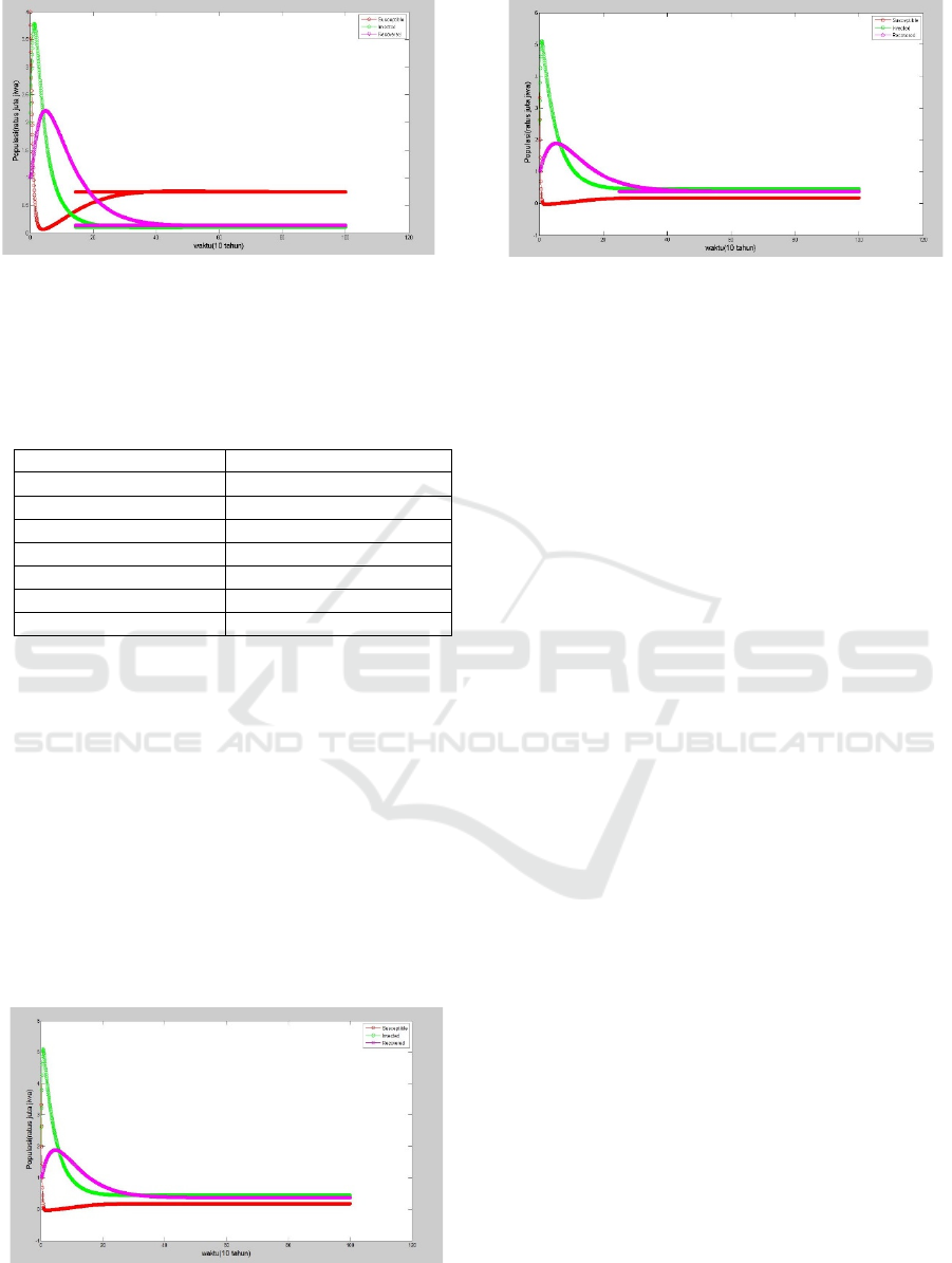
Figure 4: Simulation 1 SIRS Model R
1 with h0,07.
Then given the values for simulation 𝑅
1 with
different parameter values, the values given are as
follows:
Table 6: The parameter values simulation 2 R
1.
Paramete
r
Value
𝛼
0,008
𝛽
0,076
𝛾
0,008
𝛿
0,004
𝜇
0,0016
𝜇
0,0012
𝜇
0,0017
From the initial value and the given parameter
values obtained simulation 𝑅
1 shown in Figure 5
and 6. The population change of 𝑆 and 𝐼 is very
significant, population 𝑆 is at critical point while
population 𝐼 increases dramatically, population 𝑅
also increase, but it does not affect population 𝑆
because population 𝐼 increases very fast. When 𝑡
10 years population 𝐼 and 𝑅 decreased while
population 𝑆 increased but did not exceed population
𝐼 as in figure 5.
The graph does not reflect the behavior of the
system at a time range ℎ0.08 as in figure 6. The
following is given a table that describes the stability
of the system depends on the value of ℎ.
Figure 5:Simulation 2 SIRS Model R
1 with h0,01.
Figure 6: Simulation 2 SIRS Model R
1 with h0,07.
The graph does not show stability in the
population because ℎ is so large, the graph will be
stable if the ℎ value is less than 0.08. So, the 5th order
Runge-Kutta numerical scheme satisfies the stability
properties of the SIRS model with 𝑅
1 when the
time step sizeℎ is not greater than 0,07.
SIRS epidemic model simulation using Runge-
Kutta method of order 5 is influenced by time step
ℎ. The time step ℎ affects the time needed to
approach the equilibrium point, the greater the time
step ℎ is used the shorter the time needed to
approach the equilibrium point.
5 CONCLUSIONS
1) At condition 𝑅
1 indicates that the behavior of
the solution will be longer to point 𝐸
, which
means the longer the disease will be lost from the
population.
2) Under condition 𝑅
1 there will be an endemic
condition, where the Infected population is still in
the population, in other words the greater the rate
of transmission of the disease (𝛽 or the smaller
the cure rate (𝛼 and natural death 𝜇 cause
endemic conditions.
3) Time step ℎ affects the time required to
approach the equilibrium point in the SIRS
epidemic model using the Runge-Kutta method of
order 5, the greater the time step
ℎ
used the
shorter the time it takes to approach the
equilibrium point.
REFERENCES
Adda, P., & Bichara, D. (2012). Global Stability for SIR
and SIRS Models with Differential Mortality.
International Journal of Pure and Applied
Mathematics, 80(3), 425–433.
IMC-SciMath 2019 - The International MIPAnet Conference on Science and Mathematics (IMC-SciMath)
380

Sinuhaji, F. (2015). Model Epidemi SIRS dengan Time
Delay. Jurnal Visipena, 6(1), 78–88.
Steven, C. (2017). Applied Numerical Methods with
MATLAB for Engineers and Scientists. The McGraw-
Hill Companies.
Tulus. (2012). Numerical Study on the Stability of Takens-
Bogdanov systems. Bulletin of Mathematics, 4(1), 17–
24.
Xiaobin, R., Fanrong, M., Zhixiao, W., Guan, Y., &
Changjiang, D. (2018). SPIR: The potential spreaders
involved SIR model for information diffusion in social
networks. Physica A: Statistical Mechanics and its
Applications. Physica A: Statistical Mechanics and Its
Applications, 506, 254–269.
Stability Analysis of the SIRS Epidemic Model using the Fifth-order Runge Kutta Method
381
