Forecasting the Amount of Cough Drug Productions using Double

Exponential Smoothing Brown Method in

PT Mutiara Mukti Farma 2019

Suyanto

and Reynold Sitorus

Department of Mathematics, Faculty of Mathematics and Natural Sciences, Universitas Sumatera Utara, Medan, Indonesia

Keywords: Double Exponential Smoothing Brown Forecasting Method, Monte Carlo Simulation.

Abstract: Forecasting is an important first step in making planning for each business organization and for any

significant management decision making. Double Exponential Smoothing Brown forecasting method is one

of the time series forecast data models that is designed for a data that contains trend elements. In this study

data on the amount of drug production at P.T. Mutiara Mukti Farma from 2006 to 2018 indicated a trend

data as time goes on. The data obtained is then analyzed using a scatter diagram to determine the pattern

then analyzed using the Double Exponential Smoothing Brown method, to find the smallest forecast error

based on the smallest Mean Absolute Percentage Error (MAPE). The best α parameter value used to

forecast the amount of drug production is 0,5 with percentage error 0,08% with the form of the forecasting

equation F

(

t + m) = 425.194,8 + 3761,963m.

1 INTRODUCTION

At this time almost all companies engaged in

industry are faced with a problem that is an

increasingly competitive level of competition.

Therefore companies are required to plan or predict

the right amount of production in order to meet

market demand on time and with the appropriate

amount and will be able to meet the needs of

consumers. To be able to present the right amount of

products to consumers, of course a company is

required to have a good forecasting model.

P.T. Mutiara Mukti Farma is a manufacturing

company engaged in the pharmaceutical processing

sector. In conducting its production, the company

does not have an objective forecasting model so that

sometimes the company’s product inventory is

insufficient for consumer demand and at times

experiences overstock.

There are two types of forecasting approaches:

qualitative and quantitative. Some forecasting

techniques try to project historical experience into

the future in the form of time series. Exponential

Smoothing is one of the time series predictions.

Exponential smoothing was proposed in the work of

Robert G. Brown as a research operations analyst for

the US Navy during World War II. In 1950s, Brown

modified exponential smoothing for discrete data

and developed methods for trends and seasons. Now,

this technique has been widely used for forecasting

purposes (Karmaker et al., 2017).

A study using Double Exponential Smoothing

Brown in predicting Turkey’s dry wine (raisin)

exports predicted that exports of dried grapes

(raisins) would decrease in the coming years. A time

series flow is made to determine the trend of the

level of raisin exports from 1982 to 2015. Based on

the analysis, raisin exports in the next five years will

decrease by around 3611 tons. This study provides

information for strategic planners, international

executives and export management of traditional

Turkish agricultural products (Uysal & Karabat,

2017).

2 LITERATURE REVIEW

2.1 Definition and Concepts of

Forecasting

Forecasting is a calculation analysis technique that is

carried out using both qualitative and quantitative

approaches to estimate future events using reference

data in the past. Forecasting (forecasting) is the art

346

Suyanto, . and Sitorus, R.

Forecasting the Amount of Cough Drug Productions using Double Exponential Smoothing Brown Method in P.T. Mutiara Mukti Farma 2019.

DOI: 10.5220/0010182300002775

In Proceedings of the 1st International MIPAnet Conference on Science and Mathematics (IMC-SciMath 2019), pages 346-349

ISBN: 978-989-758-556-2

and science of predicting future events. This can be

solved by involving historical data retrieval and

projecting it into the future with a form of

mathematical model

(Heizer & Render, 2009).

2.2 Forecasting Functions and

Purposes

The forecasting function is seen when making a

decision. A good decision is a decision based on

consideration of what will happen when the decision

is implemented. If the prediction is not precise, then

forecasting problems are also a problem that is

always faced (Al Rahamneh, 2017). Forecasting has

the objective to review current and past company

policies and see the extent of influence in the future

(Heizer & Render, 2009).

2.3 Forecasting Techniques

Qualitative forecasting is forecasting techniques

used when past data are not available or available

but the amount is not much. Qualitative techniques

are based on a common sense approach in filtering

information into useful forms. Quantitative

forecasting methods are forecasting that is based on

manipulating available historical data adequately

and without intuition or subjective judgment of the

person making the forecast

(Makridakis et al., 2003).

2.4 Smoothing Method

Smoothing Method is the method of forecasting by

smoothing past data, which is to take an average of

several years take forecast value the next few years

(Hyndman et al., 2002). The general formula of the

exponential smoothing method is:

𝐹



𝛼𝑋







𝑖𝛼



𝐹



(1)

with:

𝐹



= forecast for the next period

𝑋

𝑡

= actual data in t period

𝐹

𝑡

= forecast t period

𝛼

= smoothing parameters

If the general formula is expanded it will change to:

𝐹



𝛼𝑋







𝑖𝛼



𝑋



⋯

𝛼



𝑖𝛼





𝑋









(2)

2.5 Brown’s Double Exponential

Smoothing

According to Makridakis et al., (2003) Brown’s

Double Exponential Smoothing is a linear model

proposed by Brown. This method is used when data

shows a trend. A trend is a smoothed estimate of the

average growth at the end of each period

(Makridakis et al., 2003).

The rationale for Double Exponential Smoothing

from Brown is similar to Double Moving Average

because both Single Smoothing and Double

Smoothing values lag behind the actual data when

there is an element of trend (Noeryanti et al., 2012).

Difference between Single Smoothing value and

Double Smoothing value (𝑆





𝑆





) can be added

with single smoothing value (𝑆





) and adjusted for

trend. This method uses two smoothing stages with

the same parameter, that is α. α values is between 0

and 1. The steps in using Double Exponential

Smoothing from Brown are as follows:

1. Determine single smoothing value (𝑆





)

𝑆





𝛼𝑋







1𝛼



𝑆





(3)

2. Determine double smoothing value (𝑆





)

𝑆





𝛼𝑆









1𝛼



𝑆





(4)

3. Determine the smoothing constant value (𝑎



)

𝑎



2𝑆





𝑆





(5)

4. Determine the smoothing constant value (b

)

𝑏





𝛼

1𝛼

𝑆





𝑆





(6)

5. Determine the forecast value for next period

t+m

)

𝐹



𝑎



𝑏





𝑚



(7)

and b

values can be taken at the last

observation value forecast calculation and m is

the number of periods to be predicted.

To be able to use the formula, values 𝑆





and 𝑆





must be available. But when t = 1, these values are

not available. Because these values must be

determined at the beginning of the period, to solved

this problem can be done by setting 𝑆





and 𝑆





same

with X

value (actual data)

(Makridakis et al., 2003).

2.6 Measuring Forecasting Accuracy

Mean Absolute Percentage Error

(MAPE)

MAPE or mean absolute percentage error is the

average of the total error percentage (difference)

between the actual data and the result forecasting

data. The formula for calculating MAPE is as

follows:

𝑀𝐴𝑃𝐸  

𝑃𝐸



𝑁





(8)

Percentage error of forecast:

𝑃𝐸 

𝑋



𝐹



𝑋



 100

(9)

with:

Forecasting the Amount of Cough Drug Productions using Double Exponential Smoothing Brown Method in P.T. Mutiara Mukti Farma 2019

347

= error t period

= actual data t period

= forecast value t period

N = times period

3 METHODOLOGY

The type of data used in this study is premier data

and secondary data. Premier data was obtained from

interviews using a list of questions shown to the

Production Manager. Secondary data were obtained

from production data, the data on the amount of

Omegrip cough production from 2006 to 2018. Then

based on the amount of production data, the data

was processed using quantitative forecasting

methods, time series forecasting, namely Double

Exponential Smoothing Brown, by looking at the

value the resulting error is the Mean Absoute

Percentage Error (MAPE) value. The smaller the

MAPE value generated, the more accurate the

forecast method.

4 RESULTS AND DISCUSSION

The data used in analyzing the data is the amount of

production data of the Omegrip branded cough from

2006 to 2018 P.T. Mutiara Mukti Farma Medan.

Table 1: Amount of Production of Cough Omegrip

P.T.Mutiara Mukti Farma Medan in 2006 to 2018.

Yea

Amount of Production

2006 343.000

2007 352.000

2008 361.000

2009 339.000

2010 371.000

2011 406.000

2012 393.000

2013 408.000

2014 418.000

2015 429.000

2016 425.000

2017 404.000

2018 430.000

Source: P.T. Mutiara Mukti Farma

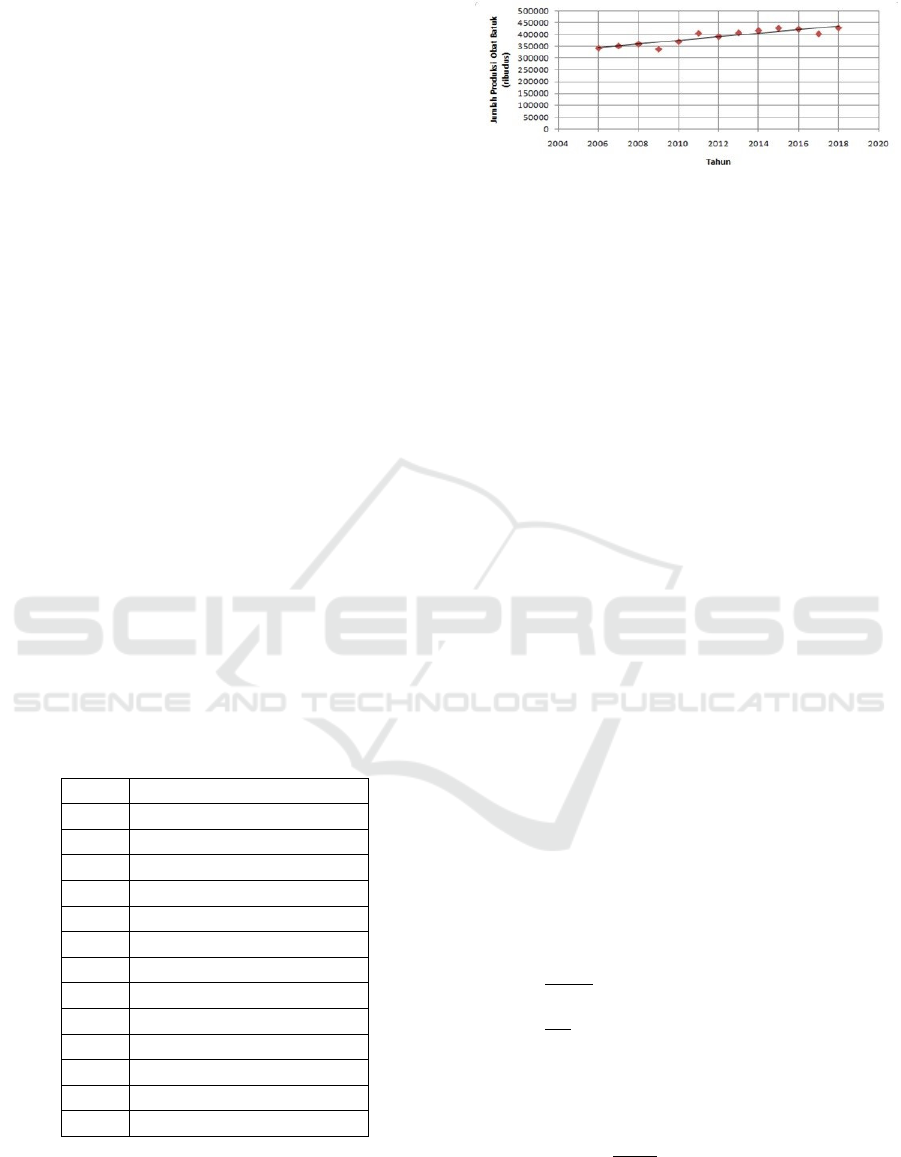
Figure 1: Data Plots for the Amount of Cough Drug

Production from 2006 to 2018.

From the plot of Figure 1 it is known that the

data obtained fluctuates. This shows that the data is

not constant. In addition to the data plots that have

been presented, it can be seen that the data has

varying data peaks but tends to increase. This shows

that the data contains trend elements, so that it can

be analyzed using Brown’s Double Exponential

Smoothing Method (Padmanaban et al., 2015).

1. For the first year (2006):

𝑆





 Determined by the amount of omegrip

cough production in the first year (2006)

that is 343,000 boxes

𝑆





 Determined by the amount of omegrip

cough production in the first year (2006),

that is 343,000 boxes, because for t − 1

values not yet obtained.

2. For the second year (2007):

𝑋



 352.000

Determine single exponential value 𝑆





𝑆





𝛼𝑋







1𝛼



𝑆





0,1



352.000







0,9



343.000



 343.900

Determine double exponential value 𝑆





𝑆





𝛼𝑆









1𝛼



𝑆





0,1



343.900







0,9



343.000



 343.090

Determine 𝑎



value

𝑎



2𝑆





𝑆





2



343.900



 343.090

 344.710

Determine 𝑏



value

𝑏





𝛼

1𝛼

𝑆





𝑆







0,1

0,9



343.900  343.090



90

Determine Mean Absolute Percentage Error

value (MAPE)

𝑀𝐴𝑃𝐸  

𝑃𝐸



𝑁





 68,4316311%

 6,22%

IMC-SciMath 2019 - The International MIPAnet Conference on Science and Mathematics (IMC-SciMath)

348

4.1 The Best 𝜶 Parameter Selection

Based on Table 2 it can be seen that the value of the

α parameter which gives the smallest Mean Absolute

Percentage Error (MAPE) value is a α = 0,5, so that

further forecasting can solved using Brown’s Double

Exponential Smoothing Brown method with the

parameter α = 0,5.

Table 2: MAPE Values for Parameters α = 0,1 to α = 0,9.

Parameter

𝛼

0,1 0,2 0,3 0,4 0,5

MAPE

6,22

2,72

1,08

0,36

0,08

Parameter

𝛼

0,6 0,7 0,8 0,9

MAPE

0,92

0,95

0,09

1,11

4.2 Forecast Result

Then to determine forecasting in the next year the

formula is used F

t+m

= a

(m) and b

value can take

2018. Because the year to be predicted is 2019, the

number of forecasting things to come is determined

by the number of the previous year. The following

are the steps for completing forecasting for 2019.

+m = a

+ b

(m)

2018+1 = a2018 + b2018

2019 = 425.194,8 + 3.761,963

2019

≈ 428.957.

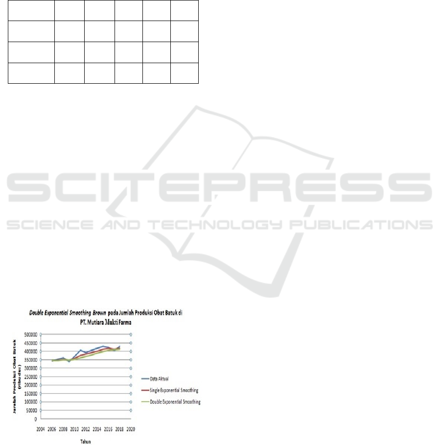
Based on the graph Figure 2 can be seen that

after smoothing twice the actual data, the graph that

will be generated will look more smoother than the

actual data graph.

Figure 2: Graph of Brown’s Double Exponential

Smoothing with α = 0,5, on the data of the amount of

Cough production in P.T. Mutiara Mukti Farma.

5 CONCLUSION

5.1 Conclusion

Based on the analysis and discussion that has been

done, it can be concluded that the best α parameter

obtained for forecasting the amount of cough

production in P.T. Mutiara Mukti Farma from 2006

to 2018 is α = 0,5 with a percentage error of 0.08%,

which results in a prediction equation F

(

t + m) =

425.194,8 + 3761,963m.

5.2 Next Research

To further research in analyzing forecasting can be

added other variables that support the forecasting of

the amount of drug production, such as factors that

affect the level of production so as to maximize the

work of the analysis of this system.

REFERENCES

Al Rahamneh, A. A. A. (2017). Using Single and Double

Exponential Smoothing for Estimating The Number of

Injuries and Fatalities Resulted From Traffic

Accidents in Jordan (1981-2016). Middle-East Journal

of Scientific Research, 25(7), 1544–1552.

https://doi.org/10.5829/idosi.mejsr.2017.1544.1552

Heizer, J., & Render, B. (2009). Manajemen Operasi Buku

1 (9th ed.). Salemba 4.

Hyndman, R. J., Koehler, A. B., Synder, R. D., & Grose,

S. (2002). A stateframework for atomatic forecasting

using exponential smoothing Methods. International

Journal of Forecasting, 18(3), 439–454.

Karmaker, C. L., Halder, P. K., & Sarker, E. (2017). A

Study of Time Series Model for Predicting Jute Yarn

Demand. International Journal of Industrial

Engineering, 1–8.

Makridakis, S., Wheelwright, S. C., & McGee, V. E.

(2003). Forecasting: Methods and Applications.

Noeryanti, Oktafiani, E., & Andriyani, F. (2012). Aplikasi

Pemulusan Eksponensial Brown dan Holt untuk Data

yang Memuat Trend. Prosiding Seminar Nasional

Aplikasi Sains Dan Teknologi.

Padmanaban, K., Supriya, Dhekale, B. S., & Sahu, P. K.

(2015). Forecasting Of Tea Export from India – an

Exponential Smoothing Techniques Approach.

International Journal of Agriculture Science, 7(7),

577–580.

Uysal, H., & Karabat, S. (2017). Forecasting and

evaluation for raisin export in turkey. Bio Web of

Conferences, 9, 1–4.

https://doi.org/10.1051/bioconf/20170903002

Forecasting the Amount of Cough Drug Productions using Double Exponential Smoothing Brown Method in P.T. Mutiara Mukti Farma 2019

349