Mathematical Methods for Controlling the Performance of an

Industrial Park

Esther S. M. Nababan, Agus Salim Harahap and Normalina Napitupulu

Department of Mathematics, Faculty of Mathematics and Natural Sciences, Universitas Sumatera Utara, Medan, Indonesia

Keywords: Carrying Capacity, Control, Robust, Environmental Performance, Performance Measurement.

Abstract: Robust reliable performance metrics enable a management to identify and address deficiencies and control

factors to improve performance of any system. The complexity of modern operating environments presents

real challenges to developing equitable and accurate performance metrics. This paper presents literature

review and analysis of how mathematical methods utilized and functioned to develop a control factor or

dynamic constraint in endeavoring to increase environmental performance of eco-industrial parks.

Constrained minimax optimization model is developed to maximize economic gain while minimizing waste

in a region within the border where dynamic carrying capacity is maintained stable. Carrying capacity is

added in as control factor to increase environmental performance within a boundary or area within which

balance of carrying capacity is maintained, in order to increase environmental performance without

reducing quality of environment.

1 INTRODUCTION

Controlling is a central notion in several academic

disciplines, but the concept has been almost

exclusively subject specific. One of the most

essential qualities required in a managing the system

or organization is that the manager of the

organization should command the respect of its’

team. This allows the manager to direct and control

all activities and the actions of the elements in the

system. Managers at all levels of management need

to perform controlling function to keep control over

activities in their areas. (McPhail et al., 2018;

Siahaan, 2011)

Therefore, controlling is very much important in

any system or organization. Controlling can be

defined as that function of management which helps

to seek planned results from the subordinates,

managers and at all levels of an organization. The

controlling function helps in measuring the progress

towards the organizational goals & brings any

deviations, and indicates corrective action. Thus, an

overall sense, the controlling function helps and

guides the organizational goals for achieving long-

term goals in future.

It is an important function because it helps to

check the errors, helps in taking the correct actions

so that there is a minimum deviation from standards

and, in achieving the stated goals of the organization

in the desired manner. According to modern

concepts, control is a foreseeing action. Whereas the

earlier concept of control was used only when errors

were detected. Therefore, controlling function

should not be misunderstood as the last function of

management. It is a function that brings back the

management cycle back to the planning function.

Thus, the controlling function act as a tool that helps

in finding out that how actual performance deviates

from standards and also finds the cause of deviations

& attempts which are necessary to take corrective

actions based upon the same. A good control system

helps an organization in accomplishing

organizational goals, judging accuracy of Standard,

making efficient use of resources, improving

employee motivation, ensuring order & discipline,

and facilitating coordination in action.

1.1 Controlling the Performance of

Industrial Park

In the industrial park, controlling the land as the

most important natural resource is conducted in

order to make optimum utilization of the natural

resources since at the certain point human beings

have caused a lot of damages to the land resources.

About 95% of our basic needs –food, clothing,

shelter come from land. Hence conservation of land

178

S. M. Nababan, E., Salim Harahap, A. and Napitupulu, N.

Mathematical Methods for Controlling the Performance of an Industrial Park.

DOI: 10.5220/0010138300002775

In Proceedings of the 1st International MIPAnet Conference on Science and Mathematics (IMC-SciMath 2019), pages 178-184

ISBN: 978-989-758-556-2

resources and development of land is extremely

crucial to the future generations can survive. There

are different land planning and conservation

measures that can be taken to protect this natural

resource such as :

a. Planting shelter belts for plants

b. Controlling over-grazing in open pastures

c. Stabilizing sand dunes

d. Proper management of wastelands

e. Controlling mining activities

f. Proper disposal of industrial waste

g. Reducing land and water degradation in

industrial areas.

Of many outcome targets of controlling, stability

is the most important outcome of controlling.

Some of them are constancy, persistence,

resilience, elasticity, amplitude, cyclical stability,

trajectory stability, global stability, local stability,

and alternate stable states (Nababan, 2014). There

are 3 basic concept of stability known in general

which are constancy, robustness and, resilience.

However, stability relates to transitions between

states. Robustness can be shown as a limiting case

of resilience, and neither constancy nor resilience

can be defined in terms of other. Hence, there are

two basic concepts of stability, both of which are

used in both the social and the natural sciences

(Nababan et al., 2017).

A performance measurement control system is

designed to help organizations improve performance

issues. Every process of a business' operations is

studied through this system to improve the

performance. When all activities have improved

performance, the organization's profitability should

increase.

1.2 Perfomance Measurement Control

System

Like many scientific concepts, fully adequate

definitions of some ecological concepts have not yet

been formulated. Performance measurement control

systems contain several key principles: All work

activity must be measured; if an activity cannot be

measured, its processes cannot be improved; all

measured work should have a predetermined

outcome regarding performance. All work activity

must be measured; if an activity cannot be measured,

its processes cannot be improved; all measured work

should have a predetermined outcome regarding

performance. Analysts (managers) determine what

the outcome of each particular activity should be. If

an activity cannot be measured, the organization

tries to eliminate it. After each activity is measured,

it is compared to the desired results. If the activity is

not performing up to the desired outcome, changes

to the activity are implemented to improve

performance. Evaluation in general is a part of all

organizations. For evaluations to be effective, the

criteria to be used for evaluation must be planned

carefully and thoroughly. Understanding the

objectives of the program and the effectiveness of

the activities carried out by the company, output

efficiency is a major component of the criteria for

evaluation (Siahaan, 2011).

To evaluate the performance of an organization,

there must be something to compare the actual

performance. Before evaluation criteria can be

developed, the goals of the organization must be

clear, especially for those who are evaluating. The

next stage is to determine whether the activity is

sufficient to meet the objectives of the organization.

The first stage of the evaluation criteria is an

investigation of the company's core operations.

These activities must be evaluated to determine

whether they are carried out correctly or not. If there

are deficiencies, management can take strategic

steps to bridge the gap to improve the entire process.

The last part of the evaluation criteria is

determining how well the activity helps the manager

achieve his goals, whether the company achieves its

objectives based on the way the activities are

regulated by the company, followed by determining

evaluation criteria is to prepare a measurement tool

to measure the efficiency of an organization's output.

This tool will consist of evaluation techniques that

measure whether a company uses its resources

wisely and in a cost effective manner and whether

objectives are met on schedule. This measurement

can help management design alternative solutions to

make company operations more efficient.

Another important part of the evaluation criteria

is studying the impact of the company. Another

important step is evaluating sustainability. This

criterion is used to determine how changes in the

competitive landscape, regulatory environment,

economic conditions, customer preferences, and the

labor market affect a company's ability to sustain

sales and profit growth. There are several

applications of control theory for a system. To

improve environmental performance, managers must

set specific goals that will improve environmental

performance.

In terms of human resource management, the

three types of control systems, namely behavioral

control, output control and input control can be used

Mathematical Methods for Controlling the Performance of an Industrial Park

179

to analyse employee behaviour and performance

(Margalef, 1969).

More advanced and more critical applications of

control concern large and complex systems the very

existence of which depends on coordinated

operation using numerous individual control devices

(usually directed by a computer). The launch of a

spaceship, the 24-hour operation of a power plant,

oil refinery, or chemical factory, and air traffic

control near a large airport are examples. An

essential aspect of these systems is that human

participation in the control task, although

theoretically possible, would be wholly impractical;

it is the feasibility of applying automatic control that

has given birth to these systems. Conceptual

representation of conditions aﬀecting ranking

stability shows that A high stability in ranking

indicates that two metrics will rank the decision

alternatives the same, whereas a low stability

indicates that two metrics will rank the decision

alternatives diﬀerently (McPhail et al., 2018).

A range of theories and methods is developed for

improving productivity in every industrial activity

without damaging the quality of the environment. A

quality of the environment can be achieved by

maintaining the ecological stability of the

environment. Each industrial activity must be carried

out within the stable region of ecological carrying

capacity. A community’s resilience stability is

determined by how fast the variable of the interest

returns to its pre-perturbed stable equilibrium.

1.3 Robustness Metric Calculation

Robustness is generally calculated for a given

decision alternative x

across a given set of future

scenarios S = {s

, s

, …, s

} using a particular

performance metric f(·).

Consequently, the calculation of robustness using

a particular metric corresponds to the transformation

of the performance of a set of decision alternatives

over different scenarios

f(x

, S) = {f(x

, s

), f(x

, s

), …, f(x

, s

)} to the

robustness R(x

, S) of these decision alternatives

over this set of scenarios. Although different

robustness metrics achieve this transformation in

different ways, a unifying framework for the

calculation of different robustness metrics can be

introduced by representing the overall

transformation of f(xi, S) into R(x

, S) by three

separate transformations: performance value

transformation (Tr.1), scenario subset selection

(Tr.2), and robustness metric calculation (Tr.3), as

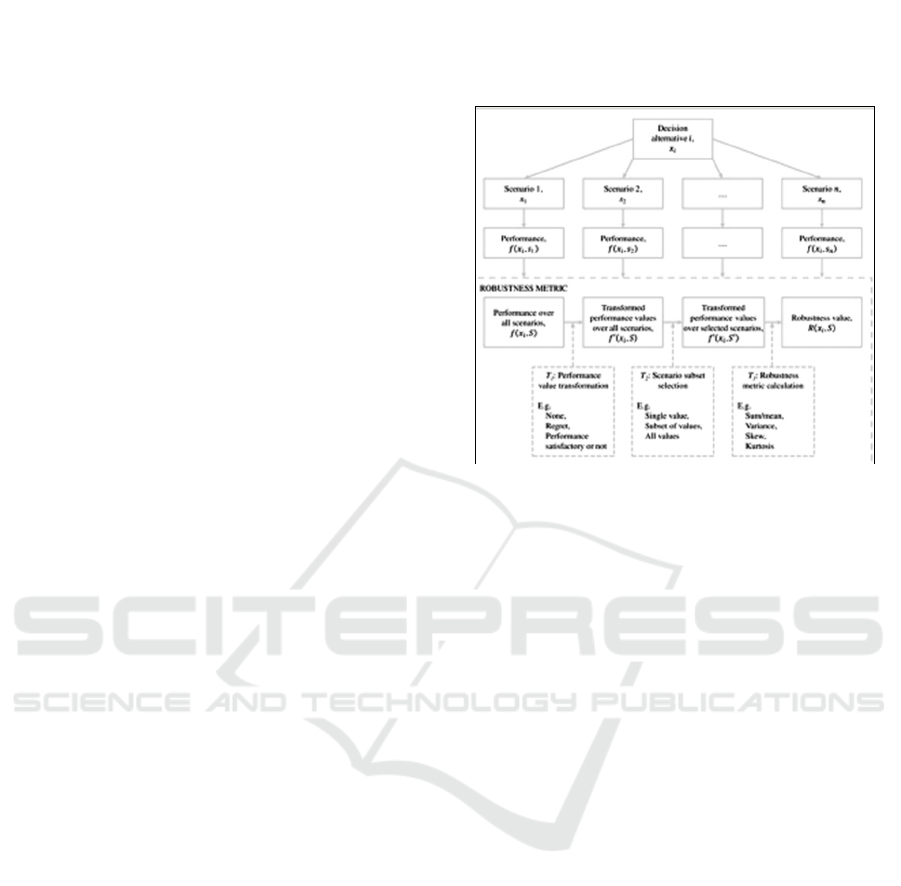
shown in Figure 1. Details of these transformations

for a range of commonly used robustness metrics are

given in Table 1 and their mathematical

implementations are given in Supporting

Information S1.

Figure 1: Unifying framework of components and

transformations in the calculation of commonly used

robustness metrics (Source: McPhail et al., 2018).

The performance value transformation (Tr.1)

converts the performance values f(xi, S) into the type

of information f′(x

, S) that is used in the calculation

of the robustness metric R(xi, S). For some

robustness metrics, the absolute performance values

(e.g., cost, reliability) are used, in which case Tr.1

corresponds to the identity transform (i.e., the

performance values are not changed). For other

robustness metrics, the absolute system performance

values are transformed into values that either

measure the regret that results from selecting a

particular decision alternative rather than the one

that performs best had a particular future actually

occurred or indicate whether the selection of a

decision alternative results in satisfactory system

performance or not (i.e., whether required system

constraints have been satisfied or not).

The scenario subset selection transformation (Tr.

2) involves determining which values of f′(x

, S) to

use in the robustness metric calculation (Tr. 3) (i.e.,

f′(x

, S′) ⊆ f′(x

, S)), which is akin to selecting a

subset of the available scenarios over which system

performance is to be assessed. This reflects a

particular degree of risk aversion, where

consideration of more extreme scenarios in the

calculation of a robustness metric that corresponds

to a higher degree of risk aversion and vice versa.

The third transformation (Tr. 3) involves the

calculation of the actual robustness metric based on

transformed system performance values (Tr. 1) for

IMC-SciMath 2019 - The International MIPAnet Conference on Science and Mathematics (IMC-SciMath)

180

the selected scenarios (Tr. 2), which corresponds to

the transformation of f′(x

, S′) to a single robustness

value, R(x

, S). This equates to an identity transform

in cases where only a single scenario is selected in

Tr. 2, as there is only a single transformed

performance value, which automatically becomes

the robustness value. However, in cases where there

are transformed performance values for multiple

scenarios, these have to be transformed into a single

value by means of calculating statistical moments of

these values, such as the mean, standard deviation,

skewness or kurtosis.

In relation to the performance value

transformation (Tr.1), which robustness metric is

most appropriate depends on whether the

performance value in question relates to the

satisfaction of a system constraint or not, and is

therefore a function of the properties of the system

under consideration. For example, if the system is

concerned with supplying water to a city, there is

generally a hard constraint in terms of supply having

to meet or exceeding demand, so that the city does

not run out of water (Beh et al., 2017). The system

performs satisfactorily if this demand is met and that

is the primary concern of the decision‐maker.

Alternatively, there might be a fixed budget for

stream restoration activities, which also provides a

constraint. In this case, a solution alternative

performs satisfactorily if its cost does not exceed the

budget. For the above examples, where performance

values correspond to determining whether

constraints have been met or not, satisficing metrics,

such as Starr's domain criterion, are most

appropriate.

In contrast, if the performance value in question

relates to optimizing system performance, metrics

that use the identity or regret transforms would be

most suitable. For example, for the water supply

security case mentioned above, the objective might

be to identify the cheapest solution alternative that

enables supply to satisfy demand. However, there

might also be concern in over‐investment in

expensive water supply infrastructure that is not

needed, in which case robustness metrics that apply

a regret transformation might be most appropriate,

as this would enable the degree of over‐ investment

to be minimized when applied to the cost

performance value. For the stream restoration

example, however, decision‐makers might simply be

interested in maximizing ecological response for the

given budget. In this case, robustness metrics that

use the identity transform might be most appropriate

when considering performance values related to

ecological response.

In relation to scenario subset selection (Tr.2),

which robustness metric is most appropriate depends

on a combination of the likely impact of system

failure and the degree of risk aversion of the

decision‐maker. In general, if the consequences of

system failure are more severe, the degree of risk‐

aversion adopted would be higher, resulting in the

selection of robustness metrics that consider

scenarios that are likely to have a more deleterious

impact on system performance. For example, in the

water supply security case, it is likely that robustness

metrics that consider more extreme scenarios would

be considered, as a city running out of water would

most likely have severe consequences. In contrast, as

the potential negative impacts for the stream

restoration example are arguably less severe,

robustness metrics that use a wider range or less

severe scenarios might be considered. However, this

also depends on the values and degree of risk

aversion of the decision maker. As far as the

robustness value calculation (Tr. 3) goes, this is only

applicable to metrics that consider more than one

scenario, as discussed previously, and relates to the

way performance values over the different scenarios

are summarized. For example, if there is interest in

the average performance of the system under

consideration over the different scenarios selected in

Tr.2, such as the average cost for the water supply

security example or the average ecological response

for the stream restoration example, a robustness

metric that sums or calculates the mean of these

values should be considered. However, decision‐

makers might also be interested in (1) the variability

of system performance (e.g., cost, ecological

response) over the selected scenarios, in which case

robustness metrics based on variance should be

used, (2) the degree to which the relative

performance of different decision alternatives is

different under more extreme scenarios, in which

case robustness metrics based on skewness should

be used, and/or (3) the degree of consistency in the

performance of different decision alternatives over

the scenarios considered, in which case robustness

metrics based on kurtosis should be used. As these

metrics are used to make decisions on outcomes, it is

important to obtain greater insight into the

conditions under which different robustness metrics

result in different decisions.

It is important to note that the relative ranking of

two decision alternatives (x

and x

), when assessed

using two robustness metrics (R

and R

), will be the

same, or stable, if the following three conditions

hold:

𝑅





𝑥





>𝑅





𝑥





and 𝑅





𝑥





>𝑅





𝑥





(1)

Mathematical Methods for Controlling the Performance of an Industrial Park

181

or 𝑅





𝑥





<𝑅





𝑥





and 𝑅





𝑥





<𝑅





𝑥





, (2)

or 𝑅





𝑥





=𝑅





𝑥





and 𝑅





𝑥





=𝑅





𝑥





(3)

𝑅





𝑥





>𝑅





𝑥





and 𝑅





𝑥





<𝑅





𝑥





(4)

or 𝑅





𝑥





<𝑅





𝑥





and 𝑅





𝑥





>𝑅





𝑥





. (5)

The relative rankings will be different or

“flipped” if the following two conditions hold:

Consequently, relative differences in robustness

values obtained when different robustness metrics

are used are a function of (1) the differences in the

transformations (i.e., performance value

transformation (Tr.1), scenario subset selection

(Tr.2), robustness metric calculation (Tr.3)) used in

the calculation of Ra and Rb and (2) differences in

the relative performance of decision alternatives x

and x

over the different scenarios considered. In

general, ranking stability is greater if there is greater

similarity in the three transformations for R

and R

and if there is greater consistency in the relative

performance of x

and x

for the scenarios

considered in the calculation of Ra and R

, as shown

in the conceptual representation in Figure 4. In fact,

if the relative performance of two decision

alternatives is the same under all scenarios, the

relative ranking of these decision alternatives is

stable, irrespective of which robustness metric is

used.

2 ECOLOGICAL STABILITY AS

A CONTROL

Ecological Indicator is a measure, or a collection of

measures, that describes the condition of an

ecosystem or one of its critical components.

Ecological indicators are used to communicate

information about ecosystems and the impact human

activity has on ecosystems to groups such as the

public or government policy makers.

Some theories define that good ecological

indicators should:

• reflect something basic and fundamental to the

long-term economic, social or environmental

health of a community over generations.

• be understood and accepted by the community as

a valid sign of sustainability or symptom of

distress

• have interest and appeal for use by local media in

monitoring, reporting and analysing general

trends toward or away from sustainable

community practices; and

• be statistically and practically measurable in a

geographical area, preferably comparable to

other cities/communities, and yield valid data.

The basic principles of developing indicators are:

use existing data, re-evaluate underlying

assumptions, integrate long-term focus with short-

term change, relate indicators to individual and

vested stakeholders, identify the direction of

sustainability, present indicators as a whole system

and determine linkages. It is also important to use a

simple and easy to understand format for presenting

data so that decision makers or other stakeholders

can base on the existing data to seek further

information that addresses issues of primary

concerns in the community.

There are the number of options for formulating

a complex definition of ecological stability.

Adopting ecological stability defined as the ability

of an ecosystem to resist changes in the presence of

perturbations, in the context of stability on industrial

parks, perturbations consists of social, economic,

environmental and political influence on the

management of industrial park (May, 1973).

Assume X

= social perturbation ; X

economic perturbation ; X

= environmental

perturbation , and X

= political perturbation. All

vectors are confined within some closed arbitrary

boundary.

Probability

1)(



(6)

Each variables can either be independently

affects the stability of industrial park, or have

simpal causal relationship or dependence among

each vectors as well as sub vectors.

By adopting Rutledge’s concepts about

ecological stability, to develop an index for the

stability a model diagram can be developed to

describe the dependence on time for each

perturbation component. All the compartment

model diagram has a dependence on time. Hence,

each main component is represented at two arbitrary

times t

and t

Let Q

be the initial conditions of the industrial

park at time t

. P

is the conditions of the industrial

parks at time t

, f

is the percentage of the total

perturbation flow through the i

component that

passes to the j

component between times t

and t

The Q

and P

refer to component of perturbation

occurs at different times with any difference in

these components and subcomponents therein

accounted by f

. The relationship between these

variables is provided by the equation :



iijj

QfP

(7)

IMC-SciMath 2019 - The International MIPAnet Conference on Science and Mathematics (IMC-SciMath)

182

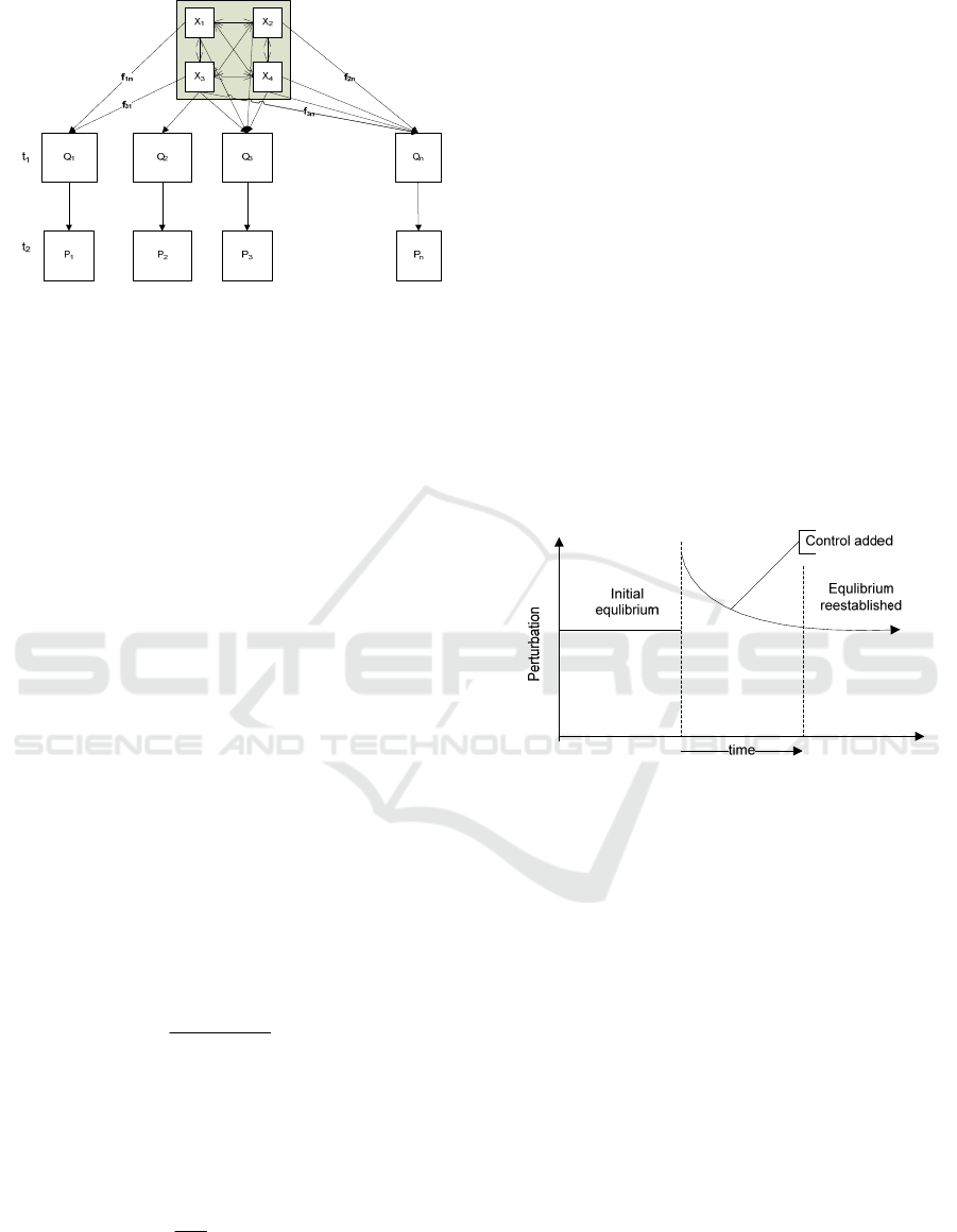
Figure 2: Diagram of main components from the original

conditions to perturbed conditions.

Perturbation flow in an industrial park ecosystem

is a fuction of time. It can occur either in a pathways

between entities or in a resources point itself

affected by internal or external perturbation. The

variables X

can be defined to be of discrete or

continue in nature which represent perturbation

flows over some arbitrary time period.

Let a

be the passage of a given increment of

perturbation through the k

component at time t

and

the b

represent the passage of a given increment of

perturbation through the j

component at time t

The diversity of the ecosystem in terms of its

throughput is given by :



−=

)(log)(

aPaPD

(8)

Where the event a

is defined as the passage of a

given increment of perturbation through the k

component and P(Q

) is the probability that event a

occured. The diversity is a function of time, since

the perturbation flow in an ecosystem is a function

of time. Hence, the time dependent nature is

obtainded by defining the appropriate events of

perturbation occurence as functions of time.

is the logarithm of the ratio of a posteriori to a

priori probabilities (Gallagher, 1986).

)(

)/(

log);(

baP

baI =

(9)

Uncertainty as measured by equation (4) is

equivalent to the uncertainty resolved about the

occurence of perturbation event b

by the occurence

of perturbation event a

(Gallagher, 1986) and is

given by :

baI log);( =

(10)

Since the complexity of the symbiotic chain

reflects the opportunities for choice of pathways, a

measure of choice is an appropriate index for

symbiotic chain and hence for ecological stability. If

one of the components is perturbed, the extent to

which it is affected may serve as an index of its

ecological stability. As perturbation occurance is a

function of time, equlibrium will dinamically change

depend on time as well. Continuous perturbation

may lead to the occurance of phase distribution

equilibrium.

For every perturbation passing through a

component in an ecosystem, a probability

assignment can be made to its destination or source.

Given a specific perturbation has passed through the

component, P(Q

) is the probability that the

increment of perturbation will affect or taken up by

the j

componen, P(Q

) is the probability that the

perturbation passed from the k

component to the j

component. The occurence of perturbation b

changes the probability of the occurence of

perturbation a

from the a proiri probability, P(Q

) to

the a posteriori probability P(Q

Figure 3: A control is added to get equilibrium

reestablished.

A quantitative measure of the uncertainty about

the occurence of perturbation events. Phase

distribution equilibrium occurs when the

perturbation event occurs continuously.

Continuous perturbation may occured by

temperature, energy flow, and chemical reactions.

Equilibrium change dinamically continuous. In such

case, equilibrium constant can is calculated on each

defined phase. Phase can either be time period, or

symbiotical phase.

One of the many ways to get the community

equilibrium reestablished is to add control. If control

is added while the system is at equilibrium, the

system must respond to counteract the control. The

system must consume the control and produce

products until a new equilibrium is established.

Mathematical Methods for Controlling the Performance of an Industrial Park

183

3 CONCLUSION

Ecological stability of industrial parks can be used

as a control developed based on choice of pathways

for symbiotic structure. Ecological stability is one of

the many indicators that affect the environmental

performance of industrial estates. This ecological

stability can be functioned as an environmental

performance control system, including the industrial

estate system. The robust method is used to

determine whether a decision alternative performs

satisfactorily under diﬀerent scenarios, and are

commonly referred to as satisﬁcing metrics.

In robust optimization, the set of uncertainties for

parameters determines a very important role. To date

there are no clear provisions on how to determine

the set of uncertainties correctly. Robust

optimization is to reduce optimal portfolio

sensitivity due to uncertainty in estimating mean

vectors and variance-covariance matrices.

Relationships among ecological stability,

diversity and complexity consistent with observed

behavior during succession arise naturally in the

development of the stability index. Theoretical

community ecology can provide a much needed

resource even when it does not give definitive

answers about what to do in particular cases but only

explores possibilities. There are a variety of stability

concepts and ecologists have begun to

systematically explore and use them to remove

various confusions concerning the complexity-

stability hypotheses.

REFERENCES

Beh, E. H. Y., Zheng, F., Dandy, G. C., Maier, H. R., &

Kapelan, Z. (2017). Robust Optimization of Water

Infrastructure Planning under Deep Uncertainty using

Metamodels. Environmental Modelling & Software,

93, 92–105.

https://doi.org/https://doi.org/10.1016/j.envsoft.2017.0

3.013

Gallagher, S. (1986). Body Image and Body Schema.

Journal of Mind and Behavior, 7, 541–554.

Margalef, R. (1969). Diversity and Stability in Ecological

Systems, G. M. Woodwell and H. H. Smith, eds.

May, R. (1973). Stability and Complexity in Model

Ecosystems. Princeton University Press.

McPhail, C., Maier, H. R., Kwakkel, J. H., Giuliani, M.,

Castelleti, A., & Westra, S. (2018). Robustness

Metrics: How Are They Calculated, When Should

They Be Used and Why Do They Give Different

Results? Resilient Decision-Making for a Riskier

World, 6(2), 169–191.

https://doi.org/https://doi.org/10.1002/2017EF000649

Nababan, E. (2014). Ecological Stability of Industrial

Park. The 4th ASEAN Environmental Engineering

Conference Proceeding.

Nababan, E., Delvian, D., & Siahaan, N. M. (2017).

Environmental Performance Indicators of Oleo-

Chemical Based Industrial Park in Indonesia: The

Conceptual Model. International Journal of Applied

Engineering Research, 12(21), 11614–11623.

Siahaan, N. (2011). Controlling Residential Supporting

Environment System to Reduce CO2 Emissions in

Urban Housing. Proceeding of the 4th ASEAN Civil

Engineering Conference.

IMC-SciMath 2019 - The International MIPAnet Conference on Science and Mathematics (IMC-SciMath)

184