Analysis of Ocean Thermal Energy Conversion (OTEC)
Potential using Closed-cycle System Simulation of 100 MW Capacity
in Bali Sea
Ismail Ali Hajar Aswad
1
, Nanda Annisa Okasari Yusal
2
, Haryo Dwito Armono
1
, Purwanto
2
,
Delyuzar Ilahude
3
, Liany Ayu Catherine
1
and Asfarur Ridwan
1
1
Faculty of Marine Technology, Sepuluh Nopember Institute of Technology, Surabaya, Indonesia
2
Faculty of Fisheries and Marine Sciences, Diponegoro University, Semarang, Indonesia
3
Marine Geological Research and Development Center, Bandung, Indonesia
Keywords: OTEC, Closed-cycle, Bali Sea.
Abstract: The Bali Sea is one of the body water that has OTEC potential because of its location in tropical region, thus
it has high sea surface temperatures. This research was conducted to examine temperature differences to run
the system and analyze the results of simulation of the closed-cycle OTEC system based on the simulation
results of Uehara and Ikegami (1990) as a basic reference in the installation of plants and obtain net power
produced by the cycle. The data used in this study is temperature in depth data per day during October
2008-June 2017 which downloaded from HYCOM website and vertical temperature data of CTD which is
the result of P3GL survey on 21 May 2017 -3 June 2017. Data processing was done by calculating the
differences in temperature of warm sea air on the surface and cold sea water at depth of 800 m by qualifying
the minimum difference requirement of 20
o
C. The results of temperature data processing yield the
difference in temperature minimum requirements of 20
o
C at all study area in the range of 21.895
o
C-24.7
o
C.
The parameter values in the closed cycle OTEC system obtained are the warm sea water (TWS) and cold
(TCS) temperatures of 28.4
o
C-30.36
o
C and 5.591
o
C-6.711
o
C; warm seawater pump power (PWS), cold
seawater pump power (PCS), and working fluid pump power (PWF) of 10.9596-11.521 MW, 16.0596-
16.621 MW, and 1.94-1.97 MW; and the heat transfer area in evaporator (AE), the heat transfer area in
condenser (AC), and total of heat transfer area (AT) of 0.737-1.7478 x105 m
2
, 0.9685-1.614 x105 m
2
, and
1.7058-3.3435 x105 m
2
. Net power potential of OTEC in Bali Sea has range between 70-71 MW with
maximum net power found at Point 2 of 71.041 MW with capacity of 100 MW and produce a cycle
efficiency of 0.41323 or 41.323%.
1 INTRODUCTION
Sunlight reaches the earth's surface 35-100 m (Avery
and Wu, 1994). The sea in the tropics absorbs the
sun continuously all the time causing sea surface
temperatures to vary to reach 27
o
C-29
o
C. The total
area of the world's tropical oceans totaling 60
million km
2
produces energy equivalent to 250
trillion fuels per yield (Nihous, 2005). Seas in
Indonesia with a total thermal potential of 2.5x10
23
Joules and an efficiency of 3%, can produce power
of 240,000 MW (Prabowo, 2012).
Sea Heat Energy Conversion (OTEC) is one of th
solutions in developing ocean energy by using
temperatures between the sea and the deep sea in the
tropics to produce electrical energy with a minimum
temperature difference of 20
o
C (Nihous, 2007).
Energy generated from sea heat is very suitable to be
applied in tropical regions such as Indonesia. If this
can be done effectively and on a large scale, OTEC
provides a renewable energy source that is needed to
complement various energy problems (Syamsuddin,
2015).
Various studies and OTEC studios that have
been carried out in Indonesia to date have been
carried out by Sinuhaji (2015) in the North Bali Sea
with the result of an increase in surface temperature
between 28-31°C with a difference of 24
o
C; Negara
and Koto (2016) in Karangkelong, North Sulawesi
with a potential of 100 kW; and Syamsuddin (2015)
at seven location points in Indonesia using World
Aswad, I., Yusal, N., Armono, H., Purwanto, ., Ilahude, D., Catherine, L. and Ridwan, A.
Analysis of Ocean Thermal Energy Conversion (OTEC) Potential using Closed-cycle System Simulation of 100 MW Capacity in Bali Sea.
DOI: 10.5220/0010046600130021
In Proceedings of the 7th International Seminar on Ocean and Coastal Engineering, Environmental and Natural Disaster Management (ISOCEEN 2019), pages 13-21
ISBN: 978-989-758-516-6
Copyright
c
 2021 by SCITEPRESS – Science and Technology Publications, Lda. All rights reserved
13

Ocean Atlas 2009. Previous research on the potential
of the OTEC in the Bali Sea is only theoretical and
must be further discussed to obtain the expected
results.
The goal of this research is to obtain minimum
temperature difference requirement of 20
o
C at seven
study points in the Bali Sea Waters, to obtain
minimum temperature difference requirement of
20
o
C at seven study points in the Bali Sea Waters
and to analyze the result of OTEC system simulation
closed cycle with 100MW power capacity.
2 SEA WATER TEMPERATURE
AND OTEC OVERVIEW
2.1 Vertical Distribution of Sea Water
Temperature
Solar thermal energy is absorbed by the surface
layer and penetrates the deeper sea. However, the
conduction process occurs so slowly that only a
small portion of the heat flowing in (Santos et al.,
2012). The temperature will decrease dramatically at
depths between 200-300 m to 1000 m. This
decreasing depth layer is known as a thermocline
that is thinner at low latitudes than at high latitudes.
At a depth of 300-1000 m, seawater does not change
in temperature and ranges from 0-3
o
C. It is
influenced by cold temperatures originating from the
mass of water from the poles then flowing into the
equatorial region (Santos et al., 2012) equatorial
region (Santos et al., 2012).
2.2 Ocean Thermal Energy Conversion
(OTEC)
It is a powerplant by utilizing the temperature
difference of seawater on the surface and the
temperature of the seawater where the ocean, which
covers two-thirds of the earth's surface area, receives
heat from solar radiation. This thermal energy can be
utilized by converting it into electrical energy with a
technology called Ocean Thermal Energy
Conversion (OTEC). A large amount of energy is
absorbed by the oceans in the form of heat that
comes from the sun's rays and magma located
beneath the seabed (Masutani and Takahashi, 2001).
2.3 OTEC System
The OTEC system is divided into three types,
namely open cycle, closed cycle, and hybrid cycle
(Aldale, 2017). The closed-cycle OTEC system is
more widely studied than other systems based on
various source literature. A closed-cycle requires a
turbine that is smaller than an open cycle (open-
cycle) and can increase the efficiency of the
electrical energy produced by the generator
(Masutani and Takahashi, 2001). This study will use
a closed-cycle OTEC system.
2.4 OTEC Power Calculation
The power generated from the turbine generator in
the OTEC system according to (Uehara and
Ikegami, 1990) is
𝑃

=𝑚

𝜂

𝜂

(
ℎ1 − ℎ2
)
(1)
Where
𝑃

: turbine generator power(𝑀𝑊)
𝑚

: the mass flow rate of the working
fluid(𝑘𝑔/𝑠)
𝜂

: turbine efficiency = 0.85
𝜂

: generator efficiency
ℎ1 − ℎ2 : a decrease in adiabatic heat between the
evaporator and the condenser
The net electrical power equation used is
𝑃

=𝑃

−
(
𝑃

+𝑃

+𝑃

)
(2)
Where
𝑃

: clean electric power (𝑀𝑊)
𝑃

: turbine generator power (𝑀𝑊)
𝑃

: warm sea flow pump power (𝑀𝑊)
𝑃

: cold sea water pump power (𝑀𝑊)
𝑃

: working fluid pump power (𝑀𝑊)
3 METHOD
The method used in this research is a quantitative
method. The first step is taking CTD temperature
data and collecting HYCOM temperature data by
using a data model downloaded from the website
http://ncss.hycom.Org/thredds /catalog.html with the
Net Common Data File (NetCDF) format which
used daily temperature data for 9 years (October
2008-June 2017) with a resolution of 1/12
o
and a
depth of 0-5500 m. The second step is the
processing of CTD temperature data and HYCOM
temperature data processing by using data
verification using the Root Mean Square Error
(RMSE) (Neill and Hashemi, 2018).
ISOCEEN 2019 - The 7th International Seminar on Ocean and Coastal Engineering, Environmental and Natural Disaster Management
14

𝑹𝑴𝑺𝑬=

𝟏
𝐧
(
𝐒
𝐢
𝐎
𝐢
)
𝟐
𝐧
𝐢𝟏
(3)
Where
n : number of observation
O : observation value
Si
: predictive value
Formula parameters to determine the bias values
by Neill and Hashemi (2018), as follows:
𝑏𝑖𝑎𝑠=𝑆
̅
−𝑂

(4)
3.1 Calculation of Sea Water Pump
Power and Working Fluid
To calculate sea water pump power and working
fluid is used the formulation by Uehara and Ikegami
(1990) and it can be followed this step.
The power of warm seawater pump is calculated
by the formulation as follows
𝑷
𝑾𝑺
=
𝒎
𝑾𝒔
∆𝑯
𝑾𝑺
𝒈
𝜼
𝑾𝑺𝑷
(5)
Cold sea water pump power is calculated with
the following formulation:
𝑷
𝑪𝑺
=
𝒎
𝑪𝑺
∆𝑯
𝑪𝑺
𝒈
𝜼
𝑪𝑺𝑷
(6)
Power of the working fluid pump is calculated
by the formulation as follows:
𝑷
𝑾𝑭
=
𝒎
𝑾𝑭
∆𝑯
𝑾𝑭
𝒈
𝜼
𝑾𝑭𝑷
(7)
Where
P
WS
: warm sea flow pump power (MW)
P
CS
: Cold sea water pump power (MW)
P
WF
: working fluid pump power (MW)
m
W
s : Mass flow rate of warm sea water (t/s)
m
CS
: Cold sea water mass flow rate (t/s)
m
WF
: Working fluid mass flow rate (t/s)
η
WSP
: Warm water pump efficiency
η
CSP
: Cold water pump efficiency
η
WFP
: Efficiency of the working fluid pump
∆H
WS
: The total pressure difference in Warm
water pipes
∆H
CS
: The total pressure difference in the Cold
water pipe
∆H
WF
: The total pressure difference in the
working fluid pipe
g : acceleration of gravity (m/s
2
)
3.2 Calculation of Sea Water Pump
Power and Working Fluid
In this study, the A
T
value was obtained from the
interpolation between the temperature difference
value (ΔT) from the temperature data processing and
the AT value using Uehara and Ikegami (1990).
To determine the total heat transfer area, the
following equation can be used from Uehara and
Ikegami (1990):
𝐀
𝑻
=𝐀
𝑬
+𝐀
𝑪
(8)
On the evaporator, the heat transfer area is
calculated by the formula:
𝐀
𝑬
=
𝑸
𝑬
𝑼
𝑬
(∆𝑻
𝒎
)
𝑬
(9)
To find out the value of the heat transfer rate on
the evaporator, can use the formula:
𝑸
𝑬
=𝒎
𝑾𝑭
(
𝒉
𝟏
−𝒉
𝟒
)
(10)
In the condenser, the heat transfer area is
calculated by the formula:
𝐀
𝑪
=
𝑸
𝑪
𝑼
𝑪
(∆𝑻
𝒎
)
𝑪
(11)
To find out the value of the heat transfer rate in
the condenser, can use the formula:
𝑸
𝑪
=𝒎
𝑾𝑭
(
𝒉
𝟐
−𝒉
𝟑
)
(12)
Where
A
T
: The area of heat transfer in the evaporator
(m
2
)
A
E
: The area of heat transfer in the condenser
(m
2
)
A
C
: Total heat transfer area (m
2
)
Q
E
: Heat transfer rate to the evaporator
Q
C
: Heat transfer rate to the condensor
(∆T
m
)
E
: logarithmic mean temperature differences
(LTMD) pada evaporator
(∆T
m
)
C
: logarithmic mean temperature differences
(LTMD) pada kondensor
(h
1
-h
4
) and (h
2
-h
3
) : the enthalpy value matches the
Rankine cycle
3.3 Calculation of OTEC Net Power
and Rankine Cycle Efficiency
The net power of OTEC (P
NET
) can be calculated
using equation (2). The efficiency of the Rankine
cycle (ηRan) can be calculated by the equation
𝜼
𝑹𝒂𝒏
=
𝑷
𝑮
𝑸
𝑬
(13)
Analysis of Ocean Thermal Energy Conversion (OTEC) Potential using Closed-cycle System Simulation of 100 MW Capacity in Bali Sea
15

Where
η
Ran
: Rankine cycle efficiency
P
G
: Turbine generator power (MW)
Q
E
: Heat transfer rate to the evaporator
4 RESULT AND DISCUSSION
4.1 Verification of HYCOM and CTD
Temperature Data
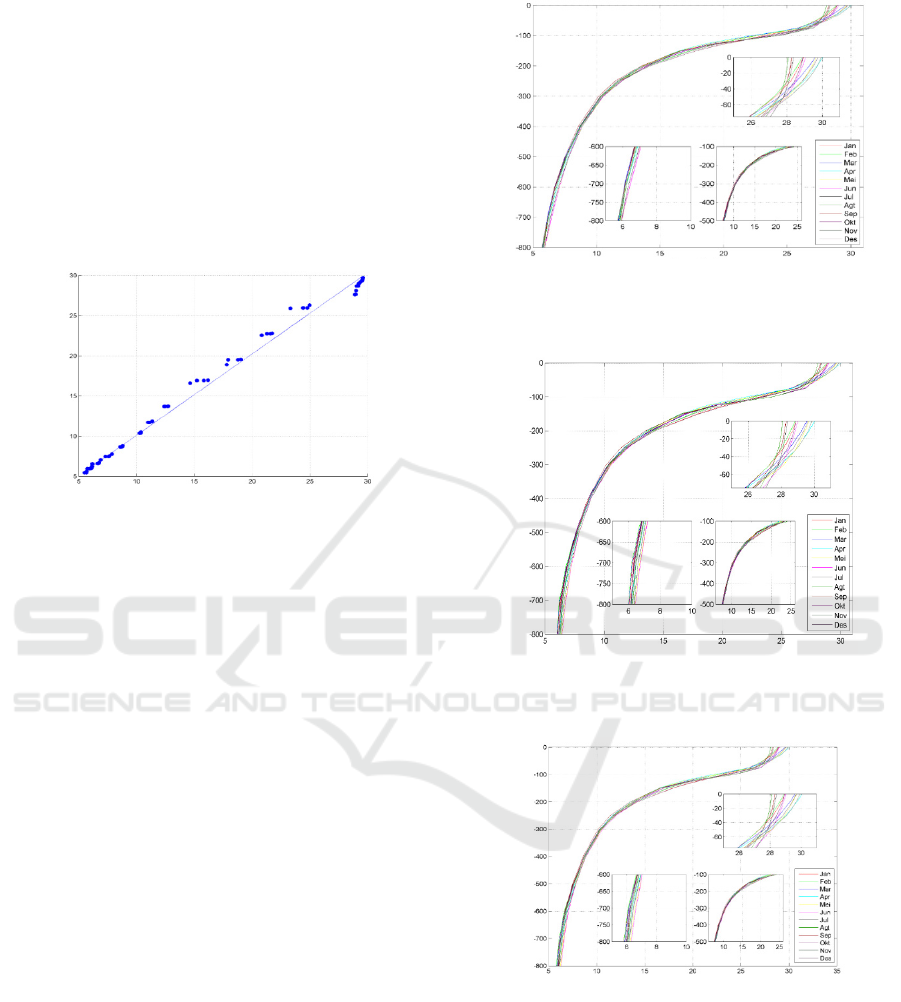
Figure 1: Distribution of Temperature Value to Depth
between HYCOM Data and C
TD
Data (Source: Data
Processing).
The error value obtained and the data distribution
graph below, then HYCOM has good data and is
considered capable of representing the temperature
conditions of the C
TD
collection.
4.2 Vertical Temperature Distribution
in the Bali Sea
The temperature of warm seawater at the surface
(T
WS
) and the temperature of cold seawater at depth
(T
CS
) are obtain to get the difference in temperature
(ΔT) between sea level and depth.
In general, temperatures that tend to be uniform
in the mixed layer (Figure 2-8) are caused by the
turbulence mechanism by wind and waves and heat
flux at sea level. Changes in temperature at the
surface of the sea and layers are mixed due to the
strength of the wind influenced by monsoons so that
the temperature at the surface of the sea and the
layers are mixed experiencing monthly variations.
Also, according to Atmadipoera and Hasanah
(2017), the temperature in the mixed layer shows
seasonal variability. The cause of this variability is
thought to be due to the influence of the mass
movement of water in the Java Sea and the Flores
Sea which partly entered the Lombok Strait.
Figure 2: Temperature Vertical Distribution Plot of 2008 -
2017 at Point 1 (Source: Data Processing).
Figure 3: Temperature Vertical Distribution Plot of 2008 -
2017 at Point 2 (Source: Data Processing).
Figure 4: Temperature Vertical Distribution Plot of 2008 -
2017 at Point 3 (Source: Data Processing).
4.3 Difference in Surface and Depth
Temperature in the Bali Sea
From 2008 to 2017, the maximum temperature
difference value occurs in April at all points as
shown in Figure 12 with the average maximum
temperature difference of 23,998
o
C. From April to
Depth (m)
Temperature (
o
C)
Depth (m)
Temperature (
o
C)
Temperature (
o
C)
Depth (m)
Temperature (
o
C)
Temperature CTD (
o
C)
ISOCEEN 2019 - The 7th International Seminar on Ocean and Coastal Engineering, Environmental and Natural Disaster Management
16

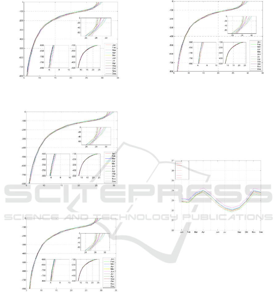
Figure 5: Temperature Vertical Distribution Plot of 2008 -
2017 at Point 4 (Source: Data Processing).
Figure 6: Temperature Vertical Distribution Plot of 2008 -
2017 at Point 5 (Source: Data Processing).
Figure 7: Temperature Vertical Distribution Plot of 2008 -
2017 at Point 6 (Source: Data Processing).
August, the temperature difference decreased quite
dramatically at all points with an average decrease
of 1,975
o
C. The lowest temperature difference
occurred in August, with an average of 22,023
o
C.
Then, starting in August there was a significant
increase of 1,933
o
C at all points until November
with an average temperature difference of 23,956
o
C
for the month.
Figure 8: Temperature Vertical Distribution Plot of 2008 -
2017 at Point 7 (Source: Data Processing).
Bali Sea meets the potential OTEC requirements
of more than 20
o
C during October 2008-2017 with a
temperature difference ranging from 21.9
o
C to
24.5
o
C. However, this potential needs to be studied
further to get the true potential by determining the
net power value based on a closed-cycle system
simulation of 100 MW.
Figure 9: Average Monthly Temperature Difference in
2008-2017. (Source: Data Processing).
4.4 Closed Cycle System Simulation
4.4.1 Warm and Cold Water Temperature
Profiles
This shows that the temperature of cold seawater is
not affected by monsoons like warm seawater
temperatures. The almost uniform temperature is
caused by a large enough density in the deep sea so
that the mass of seawater is denser. The high density
is caused by layers in the deep sea not having a
direct influence from the wind, the intensity of
sunlight, precipitation and evaporation, and cloud
cover such as the temperature of warm seawater.
Depth (m)
Temperature (
o
C)
Depth (m)
Temperature (
o
C)
Depth (m)
Temperature (
o
C)
Temperature (
o
C)
Depth (m)
Month
Temperature (
o
C)
Point 1
Point 2
Point 3
Point 4
Point 5
Point 6
Point 7
May
Aug
Analysis of Ocean Thermal Energy Conversion (OTEC) Potential using Closed-cycle System Simulation of 100 MW Capacity in Bali Sea
17

Figure 10: Variations in Surface Temperature Monthly
(T
WS
) and Temperature Depth (T
CS
) in 2008-2017 (Source:
Data Processing).
Figure 11: Monthly Variations of Warm Sea Water
Temperature on T
WS
2008-2017. (Source: Data
Processing).
Figure 12: Monthly Variations in Cold Sea Water
Temperature at Depths of 800 m (T
CS
) in 2008-2017
(Source: Data Processing).
4.4.2 Pump Power for Warm Water, Cold
Water and Working Fluid
Figure 13: Monthly Warm Water Pump Power (P
WS
) in
2008-2017 (Source: Data Processing).
Warm seawater pump power reached the highest rate
in August, which was an average of 11,495 MW.
Meanwhile, the lowest warm seawater pump power
occurred in April with an average value of 11.1
MW.
Coldwater pump power reached the highest rate
in August, which was an average of 16,595 MW.
Meanwhile, the lowest warm seawater pump power
occurred in April with an average value of 16.2
MW. Coldwater pump power is stable from year to
year with a range between 1.94-1.97 MW.
Figure 14: Monthly Cold Power Pump (P
CS
) 2008-2017
(Source: Data Processing).
Figure 15: Power of Monthly Working Fluid Pump (P
WF
)
in 2008-2017 (Source: Data Processing).
Month
Temperature (
o
C)
Temperature (
o
C)
M
o
n
t
h
Month
Water Pump Fluid Warm Water (MW)
Temperature (
o
C)
Month
Month
Month
Cold Power Pump (MW)
Fluid Pump
Point 1
Point 2
Point 3
Point 4
Point 5
Point 6
Point 7
Point 1
Point 2
Point 3
Point 4
Point 5
Point 6
Point 7
Point 1
Point 2
Point 3
Point 4
Point 5
Point 6
Point 7
Point 1
Point 2
Point 3
Point 4
Point 1
Point 2
Point 3
Point 4
Point 5
Point 6
Point 7
ISOCEEN 2019 - The 7th International Seminar on Ocean and Coastal Engineering, Environmental and Natural Disaster Management
18

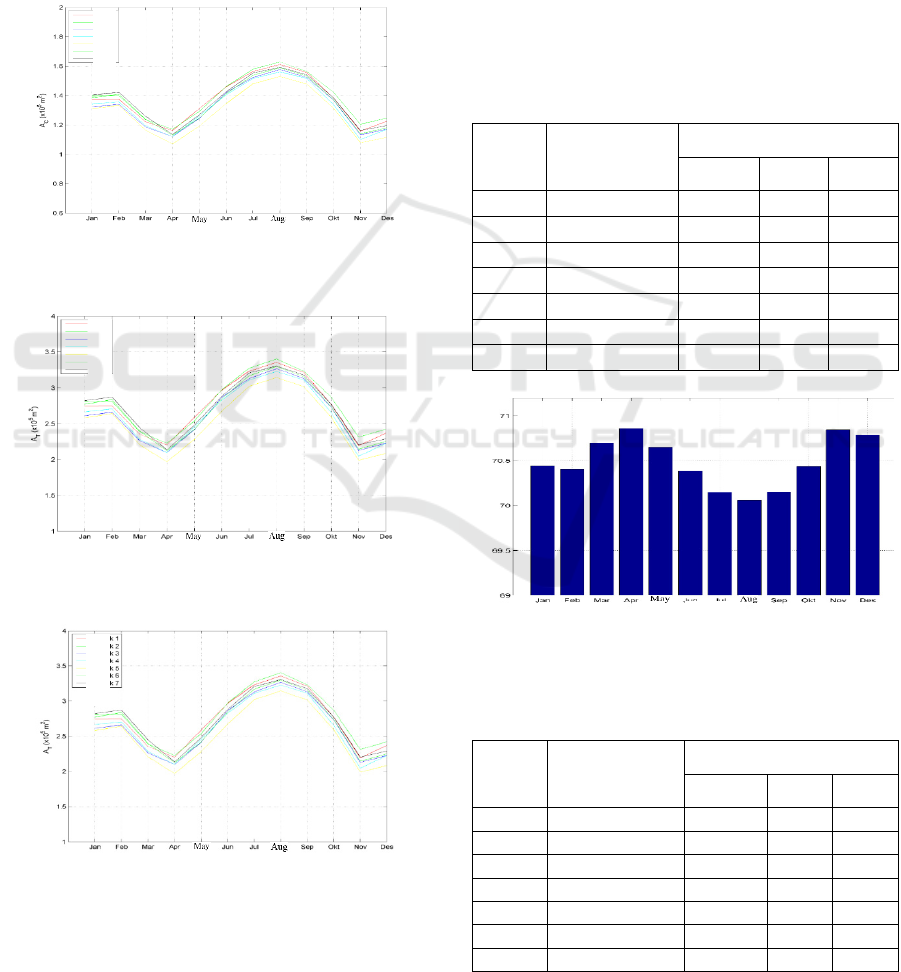
4.4.3 Heat Transfer Area
The heat transfer area in the evaporator reached the
highest number in August, which was an average of
1.70164x105m
2
. Meanwhile, the lowest heat transfer
area in the evaporator occurred in April with an
average value of 0.99052 x105m
2
.
The area of heat transfer in the condenser
reached the highest number in August, namely an
average of 1,58466 x105m
2
and the lowest in April
with an average value of 1.130330 x105m
2
.
Figure 16: Area of Heat Transfer in Monthly Evaporators
2008-2017 (Source: Data Processing).
Figure 17: Heat Transfer in Monthly Condenser (A
C
)
2008-2017 (Source: Data Processing).
Figure 18: Total Heat Transfer Area (A
T
) in 2008 -2017
(Source: Data Processing).
4.5 Calculation of OTEC Net Power
and Cycle Efficiency
The results of the OTEC net power estimation
results are listed in the table 1.
The highest net power for 9 years (Table 1.) was
achieved in April with an average net power of
70,759 MW and the lowest occurred in August with
an average net power of 69,969 MW. The maximum
cycle efficiency is 0.4061 at Point 5. The highest
cycle efficiency occurs in April with an average
maximum value of 0.402, while the lowest cycle
efficiency occurs in August with an average
minimum value of 0.3704.
Table 1: OTEC Clean Power at Study Point 2008-2017.
Location Temperature
Difference (
O
C)
Clean Power (MW)
Average Min Max
Point 1 22.969 70.348 69.922 70.711
Point 2 22.896 70.318 69.891 70.689
Point 3 23.140 70.416 69.981 70.775
Point 4 23.157 70.423 70.010 70.810
Point 5 23.327 70.491 70.064 70.863
Point 6 23.053 70.381 69.961 70.759
Point 7 22.990 70.356 69.956 70.750
Figure 19: Monthly Net Power in 2008-2017 at the
Potential Point (Source: Data Processing).
Table 2: Efficiency of the Rankine Cycle at the Study
Point in 2008-2017.
Location
Clean Power
Average (MW)
Efficiency
Average Min Max
Point 1 70.348 0.3855 0.3685 0.4000
Point 2 70.318 0.3843 0.3672 0.3992
Point 3 70.416 0.3882 0.3709 0.3026
Point 4 70.423 0.3885 0.3720 0.4040
Point 5 70.491 0.3912 0.3742 0.4061
Point 6 70.381 0.3868 0.3700 0.4020
Point 7 70.356 0.3858 0.3698 0.4016
Month
Month
Month
Clean Power (MW)
Point 1
Point 2
Point 3
Point 4
Point 5
Point 6
Point 7
Point 1
Point 2
Point 3
Point 4
Point 5
Point 6
Point 7
Point 1
Point 2
Point 3
Point 4
Point 5
Point 6
Point 7
Month
Analysis of Ocean Thermal Energy Conversion (OTEC) Potential using Closed-cycle System Simulation of 100 MW Capacity in Bali Sea
19

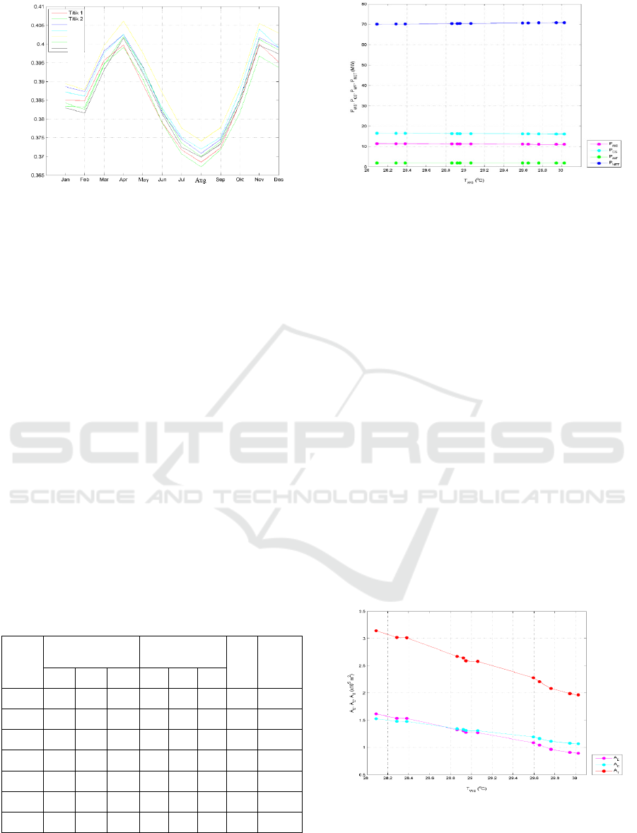
Figure 20: Efficiency of Monthly Cycles in 2008-2017
(Source: Data Processing).
4.6 Discussion of Closed Cycle OTEC
System Simulation
The power of warm seawater pumps (P
WS
) and cold
seawater pump power (P
CS
) decreases but is not very
significant, while the power of the working fluid
pump (P
WF
) is stable against the increase in T
WS
.
Meanwhile, the net power (P
NET
) increased from
70.06 MW to 70.86 MW. P
NET
value is derived from
the remaining power generated by the turbine due to
be used to pump warm seawater, cold seawater, and
working fluid.
The heat transfer area in the evaporator (A
E
)
decreases from 1.61633x105m
2
to 0.89701x105m
2
.
Likewise, the area of heat transfer in the condenser
(A
C
) which also decreased from 1.53015 x105m
2
to
1.0705882x105m
2
. This decrease certainly affects
the value of the area of heat transfer on the
condenser (A
T
) which decreased from 3.14648
x105m
2
to 1.967596 x105m
2
Table 3: Simulation Parameter Value Based on 100 MW
Closed Cycle Simulation.
Location
Pump Power (MW)
Heat Transfer Area
(x10
5
m
2
)
Net
Power
(MW)
Cycle
Efficiency
(%)
P
WS
P
CS
P
WF
A
E
A
C
A
T
Point 1 11.306 16.406 1.94 1.361 1.367 2.728 70.348 0.3855
Point 2 11.321 16.421 1.941 1.387 1.384 2.771 70.318 0.3843
Point 3 11.272 16.372 1.951 1.300 1.328 2.628 70.416 0.3882
Point 4 11.269 16.369 1.951 1.293 1.324 2.617 70.423 0.3885
Point 5 11.235 16.335 1.94 1.232 1.285 2.517 70.491 0.3912
Point 6 11.289 16.389 1.951 1.331 1.348 2.679 70.381 0.3868
Point 7 11.302 16.402 1.95 1.354 1.362 2.716 70.256 0.3858
Figure 21: Relationship Between Pump Power (P
WS
, P
CS
,
P
WF
) and Clean Power (P
NET
) (Source: Data Processing).
Uehara and Ikegami (1990) stated that the cost of
the heat exchanger is one of the components that
most cuts the cost of generation, around 25-50% of
the total cost. Therefore, it is necessary to obtain the
minimum objective function value by increasing the
production of clean electric power and the heat
exchanger needed to optimize the area of heat
transfer can be suppressed.
The graph (Figure 24.) shows a linear
relationship between net power and cycle efficiency.
Increasing the value of net power will also increase
the value of cycle efficiency. To produce a
maximum electric power of 70.86 MW, the
efficiency of the issued Rankine cycle reaches a
maximum of 0.4061 or 40.61%. The efficiency of
the Rankine cycle comes from how efficient the
OTEC generator is in releasing power to pump
warm seawater (P
WS
), cold seawater (P
CS
), and
working fluid (P
WF
). Thus, the greater the net power
produced, the pump power produced must also be
greater and this will increase the value of the
Rankine cycle efficiency.
Figure 22: Relationship Between Heat Transfer Area in
Evaporator and Condenser (A
E
, A
C
) and Total Heat
Transfer Area (A
T
) (Source: Data Processing).
Month
Cycle Efficiency (%)
Point 1
Point 2
Point 3
Point 4
Point 5
Point 6
Point 7
ISOCEEN 2019 - The 7th International Seminar on Ocean and Coastal Engineering, Environmental and Natural Disaster Management
20

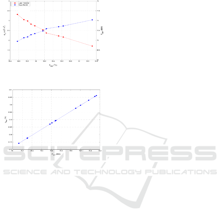
Figure 23: Relationship Between Total Heat Transfer Area
(A
T
) and Clean Electricity Power (P
NET
) (Source: Data
Processing).
Figure 24. Relationship Between Clean Electric Power
(P
NET
) and Cycle Efficiency (ηRan) (Source: Data
Processing).
5 CONCLUSION
1. Minimum temperature difference requirement
of 20
o
C at seven study points in the Bali Sea
Waters was fulfilled during 2008-2017 with a
range between 21.9
o
C - 25.3
o
C.
2. Potential net electric power OTEC in the Bali
Sea has a range between 69.8-70.8 MW with a
maximum net power found at Point 5 of 70.86
MW with a capacity of 100 MW with cycle
efficiency of 0.4061 or 40.61%.
3. Based on the simulation of closed cycle OTEC,
the components that describe and support the
potential of OTEC are warm sea water
temperature (T
WS
) and cold water (T
CS
) of 28
o
C-
30
o
C and 5.7
o
C-6.4
o
C; warm sea water pump
power (P
WS
), cold sea water pump power (P
CS
),
and working fluid pump power (P
WF
) of 11,048-
11,543 MW, 16,148-16,634 MW, and 1.94-1.97
MW; heat transfer area on the evaporator (A
E
),
heat transfer area on the condenser (A
C
), and the
total heat transfer area (A
T
) of 0,897-1,772x105
m
2
, 1,07059-1,62968x105 m
2
, and 1,9676-
3.401794x105 m
2
.
REFERENCES
Aldale, Abdullah Mohammed. 2017. “Open Access Ocean
Thermal Energy Conversion (OTEC) American
Journal of Engineering Research (AJER).” (4):164–67.
Avery, W.H. and Chih Wu. 1994. Renewable Energy from
The Ocean: A Guide To OTEC. Oxford University
Press, Inc., New York, 446 p.
Masutani. and Takahashi. 2001. “Ocean Thermal Energy
Conversion (Otec).” 1(1997):1993–99.
Negara, Ridho Bela dan J. Koto. 2016. Potential of 100
kW of Ocean Thermal Energy Conversion in
Karangkelong, Sulawesi Utara, Indonesia.
International Journal of Environmental Research &
Clean Energy, 5 (1): 1-10
Neill, Simon P., Hashemi, M. Reza. 2018. Fundamentals
of Ocean Renewable Energy: Chapter 8-Ocean
Modelling for Resource Characterization.Academic
Press. Elsevier 1
st
Edition
Nihous, Gérard C. 2007. “A Preliminary Assessment of
Ocean Thermal Energy Conversion Resources.”
Journal of Energy Resources Technology,
Transactions of the ASME 129(1):10–17.
Prabowo, H. 2012. Atlas Potensi Energi Laut. J. M&E,
10(4): 65-71.
Santos, Fran, Moncho Gómez-Gesteira, Maite deCastro,
and Inés Álvarez. 2012. “Variability of Coastal and
Ocean Water Temperature in the Upper 700 m along
the Western Iberian Peninsula from 1975 to 2006.”
PLoS ONE 7(12):2–8.
Sinuhaji, A.R. 2015. Potential Ocean Thermal Energy
Conversion (OTEC) in Bali. KnE Energy, 1: 5-12.
Syamsuddin, Mega L., Adli Attamimi, Angga P. Nugraha,
and Syahrir Gibran. 2015. “OTEC Potential in The
Indonesian Seas.” Energy Procedia 65:215–22.
Uehara, Haruo dan Yasuyuki Ikegami. 1990. Optimization
of a Closed Cycle OTEC System. Journal of Solar
Energy Engineering, 112: 247-256.
Transfer Area
Clean Power
Analysis of Ocean Thermal Energy Conversion (OTEC) Potential using Closed-cycle System Simulation of 100 MW Capacity in Bali Sea
21