The Role of International Trade to Economic Growth: The Case of

Indonesia

Hendri Tanjung

and Abrista Devi

Universitas Ibn Khaldun Bogor, Jl. KH. Soleh Iskandar,Bogor, Indonesia

Keywords: Export, Import, Economic Growth

Abstract: This study is aimed to identify the effect of export and import toward economic growth in Indonesia. Using

the monthly data from the year 1999 to 2017 and Vector Autoregression analysis, it is found that Gross

Domestik Product (GDP) will response negatively in short term and positively stable in the long term in period

of 15 due to the shocked of export. Furthermore, GDP will response positively in short term and positively

stable in the long term in period of 20 due to the shocked of import. There is no significant effect export to

GDP as well as import to GDP in the short term and long term. Therefore, there is no effect of international

trade (export and import) to economic growth for Indonesia.

1 INTRODUCTION

In the earliest 2018, several government policies

shocked Indonesian related to the food material

import. This policy remain unrest to the society

because Indonesia is popular with Agrarian and rich

with natural resources country but in fact still

importing for some food materials. Nowadays,

Indonesia still suffers from the lack of rice stock;

therefore the inflation rise due to the rice price

increased. Despite of rice, the inflation also might

happen to other food materials such as brown sugar,

salt industry, etc. Indonesia is not only importing food

materials, but also importing other products such as

gas and oil. Plethora public news highlight that

Indonesia also import labor from China. Supporting

this latter assertion of BPS year 2017, China was

dominated export and import activity in Indonesia.

Notwithstanding, Indonesia balance of trade

conditions were surplus at US$ 1.76 billion, export

were at US$ 14.54 billion and import were at US$

12.78 billion. The supernumerary of trade balance is

occurred due to the number of import were greatly

decreased compared to the number of export.

Economic sector is the most important sector to

measure the welfare of a country. We can consider

that a country is in a prosperity condition through the

number of its economic growth. Basically, if the

economic growth experience positive direction,

therefore we can say that the country is welfare, and

otherwise. There are many determinant factors

affected to the level of country’s prosperity

measurement, for example, inflation, politic situation,

etc. Be advised that papers in a technically unsuitable

form will be returned for retyping. After returned the

manuscript must be appropriately modified.

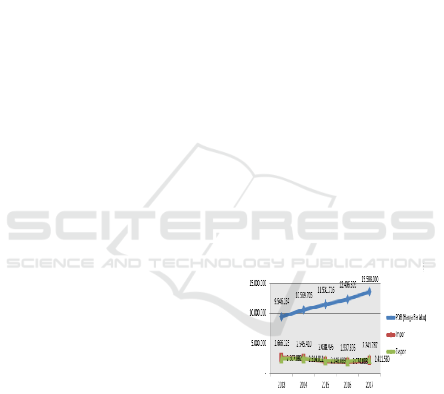
Graph 1: The GDP, Import, and Export Trend by the year

2013-2017 (IDR billion) Source: Statistic Center (2017)

The graph 1 depicts of Indonesia economic

growth trend which is reflected by GDP (Gross

Domestic Product), import and export value by the

year 2013 - 2017. According to the number of

economic growth which is represented by GDP,

Indonesia experienced a good economic growth

where GDP positively increased over time. However,

the growth of product and services produced

disproportionate with the movement of export and

2166

Tanjung, H. and Devi, A.

The Role of International Trade to Economic Growth: The Case of Indonesia.

DOI: 10.5220/0009940421662174

In Proceedings of the 1st International Conference on Recent Innovations (ICRI 2018), pages 2166-2174

ISBN: 978-989-758-458-9

import activity in Indonesia. As shown in graph 1,

export and import activity from the year 2013 to 2017

were fluctuated and tend to decreased. Specifically,

export and import experienced decreased from the

year 2014 to 2016 and start to increase in 2017.

Trade reformation has an important role to

determine the policy direction of a country. Every

country, both advanced countries and developed

countries have a very uniqueness natural resource and

tend to differ among another. This means that every

country has potency to create product with their own

comparative advantage, such as raw material, labor,

and other costs to produce the specific product

(Adeleye, Adeteye & Adewuyi, 2015). Therefore, the

existence of trading system is greatly important, not

only rely on intern trading, but also expand to the

international scale.

Import-export activity provides much benefit to

the involved-country. Export is one of foreign

exchange source that are greatly required by the open-

country or region as well as Indonesia, because a wide

export to various countries will increase the number

of production and promote the economic growth, so

it is expected to greatly contributing toward economic

stability (Rivai, 2006). Meanwhile, through import, a

country is able to fulfill their intern need that probably

cannot be produced internally or use the comparative

advantage pattern so the exceed cost of product and

services will be cheaper.

Export and import activity can support the

economic growth of a country (Roshan, 2007;

Velnampy & Achchuthan, 2013). Hye (2012) argues

in his research in China that export will lead to

economic growth of a country as well as economic

growth will lead to export. Besides, import also will

lead to economic growth as well as economic growth

will lead to import (exports-led growth, growth-led

exports, imports-led growth, and growth-led

imports). Meanwhile, plethora empirical research

revealed that despite of export, import also led to

economic growth. Hasim & Masih (2014) also

addresses the issue of import activity, where import

has an important role to stimulate the overall

economic performance of a country. The effect of

import toward economic growth may be difference

with the effect of export toward economic growth.

“The transfer of technology from developed to

developing countries through imports may serve as an

important source of economic growth. Imports can be

a channel for long run economic growth because it

provides domestic firms access to foreign technology

and knowledge.” (Hasim & Masih, 2014).

Through import, country will have opportunities

in technology and knowledge exchange among

countries, so it also will lead to the economic growth

in the long term. Supporting this latter assertion of

Mazumdar (2001) that import will led to economic

growth (import-led-growth (ILG). The source of

western knowledge also has important role toward the

growth of productivity of a country through their

technology innovations scuh as computer, machine,

and tools. So, it is fairly to conclude that import

influences the economic growth through import

competitiveness. “Imports can affect the productivity

growth through its effect on domestic innovation

through import competition. An increase in import

penetration will exposes the domestic firms to foreign

competition. Import are important to productivity

growth because the domestic producers will respond

to the technological competitive pressure from

foreign competition.”(Hasim & Masih, 2014).

As well-discussed in the previous paragraph,

export and import activity is being an important factor

which is contributing to the economic growth of a

country. Gross Domestic Product (GDP) indicator

represents the economic growth consist of 17

economic sector categories based on industry sector.

GDP value is representing the growth of society’s

economic activity who work and also the total

number of value added (product) which are produced

from various number of job employment. According

to the discussion above, the objectives of this study is

aimed to identify the effect of export and import

toward economic growth in Indonesia.

2 LITERATURE REVIEW

Boediono (1999) defines economic growth theory as

an explanation of factors which are affecting the

increasing of income per-capita in the long term. He

also argues that economic growth as an explanation

of enhancement factors among others, then the

growth process occurred. Economic growth theory is

divided into two groups: (1) classical theories,

involve the growth theory of Adam Smith, David

Richard, and Arthur Lewis. The difference between

Lewis theory and other classical theories was found

that Lewis emphasizes to the economic dualism

aspect, where the existence of modern sector and

traditional sector. Each sector has its own specific

economic characteristic. (2) Specific theories,

involve 4 (four) sub groups, namely:

a. Growth theory of Neo Classic, initiated by

Robert Solow and Trevor Swan theory

b. Optimum growth theory. This theory is

intended to seek the most optimum of

The Role of International Trade to Economic Growth: The Case of Indonesia

2167

economic growth path involve Dalil Emas

theory and Jalan Raya theory

c. Growth theory escorted by money. This is a

development theory of neo classical theory,

but by the additional of money as the wealth

property. The basic theory comes from James

Tobin masterpiece.

Nowadays, the definition of economic growth has

an extended discussion, another main issue explored

in detain in Prof. Simon Kusnets, where Jhingan

(2005) analyzes that economic growth is defined as

the increasing of country’s capability to serve a large

number of economic product variations to their

society in the long-term. This growth of this potency

is tailored to the technology development,

organization adjustment, and the ideology

requirement. This definition is divided into 3 (three)

component; (1) economic growth of a country is seen

from the persistently increasing of commodity stock;

(2) advanced technology is being a factor of

economic development where determine the growth

level of ability to serve a large number of economic

product variations to their society; (3) the using of

technology widely and efficiently is required the

adjustment of organization and ideology, so the

innovations that are generated by knowledge can be

utilized effectively.

Plethora academic research found that economic

growth affects toward international trading activity

and whereas the international trading (export and

import activity) can led to the economic growth

(Won, 2008; Shahbaz & Rahman, 2014). One of the

economic groth indicator is GDP. In the several of

academic reserarch, GDP is widely used as proxy

represents the economicy growth (Adeleye, Adeteye

& Adewuyi, 2015; Akanni, 2007; Vohra, 2001).

Gross Domestic Product (GDP) is the market value of

overall product and service, which are produced by a

country in a period of time (Kravis, Heston &

Summers, 1982). GDP is also used to calculate the

national income. GDP means the overall value of

product and service which are produced by a country

in the specific period (normally in a year).

Internationl trading involve export adn import

activity where the exchange of product and service

among countries is occured. Export is an activity

where a country sells their commodity (both product

and service) outside the coutry by utilizing the

approved-payment system between seller (exporter)

and buyer (importer). Meanwhile, import is the

purchasing activity of commodity from the outside

countries to the domestic (Seyoum, 2009).

Please remember that all the papers must be in

English and without orthographic errors. Do not add

any text to the headers (do not set running heads) and

footers, not even page numbers, because text will be

added electronically. For a best viewing experience

the used font must be Times New Roman, on a

Macintosh use the font named times, except on

special occasions, such as program code (Section

2.3.7).

3 RESEARCH METHOD

This study is conducting timeseries secondary data

which is obtained from Statistic centre (BPS/Badan

Pusat Statistik) and published in their official website

(www.bps.go.id). Data is obtained from the monthly

data from the year 1999 to 2017.

Table 1: Operational Variable Explanations

NO Variable Operational

Explanations

Source

of Data

1 GDP

(Gross

Domestic

Product)

Current price will

be used as proxy of

GDP due to more

representattive of

the real price

Statistic

Centre

2 Export Monthly export

value

Statistic

Centre

3 Import Monthly import

value

Statistic

Centre

To have better understanding of the data usability in

this research, following explanation will be

discussed:

1. GDP (Gross Domestic Product): current price is

used as proxy of GDP due to more representative

of the real price (real time). Current price is

selected rather than nominal price due to

diminisshing of inflation effect, therefore, the

value of economic growth will represent the real

condition. Monthly GDP data is obtained using

interpolation method (quadratic match sum

method) over quartile GDP with Eviews 9.

2. Export and Import: the data which is used to

represent the value of import and export is the

total number of monthly export and import by the

year 1999-2017 and can be obtained from the

official website of statistic centre

(www.bps.go.id)

The equation model that is constructed in this

model to identify the export and import contribution

toward economic growth as follows:

ICRI 2018 - International Conference Recent Innovation

2168

LnGDPt = α + βj ∑ LnEkspt-j + γj ∑ LnImpt-j

+ μ1t......(3.1)

j =1 j=1 j=1

Where:

LnExp : Natural Logarithm transformation of export

LnImp : Natural Logarithm transformation of import

LnGDP : Natural Logarithm transformation of GDP

The research problem of this study will be analyzed

by employing Vector Auto-regression econometric

technique. VAR simply describes the causality

relationship among variables in a system, by adding

intercept. Ascarya (2009) argues that this method was

developed by Sims in the year 1980 respectively.

Sims (1980) assumed that all variables are

endogenous (determined in the model), therefore this

method is named by e-theoretic model (without

theoretical based). If the used data is stationer in the

first difference, then VAR model will be combined by

the correction model so we called as Vector Error

Correction Model (VECM). Impulse response

function analysis will be conducted to identify the

response of endogenous variables toward the shock of

other variables in the model. Variance

decomposititon analysis also will be conducted to

explain the variability of endogenous variables

(Tanjung & Devi, 2013). The entire data of this study

is transformed to the natural logarithm form (LN

form). The software employs in this study is

Microsoft Excel and Eviews 9.

VAR method provides the convenience to use

and also minimizes the lack to determine the

endogenous and exogenous variables. There are

several benefit provided by VAR (Gujarati, 2003):

1. Easy to estimate, Ordinary Least Square (OLS)

method can be applied to each different equation

separately.

2. Better estimation of forecasting rather than

complexity simultaneous equation model.

3. Impulse Response Function (IRF) provides the

response from dependent variable in the VAR

system toward shock of error term.

4. Variance Decomposition provides information

regarding to the importance of each error term to

influence all variables in VAR.

The step of research using VAR analysis will be

explained as follows

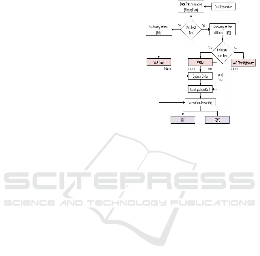
Figure 1: VAR Step of Research

Source: Ascarya, et al. (2008

Figure 1 describes the steps of research where

provides different information comply with the

characteristic of result. If data is stationer in VAR

level, this means that the data contains long-term

information. While, if data is non-stationer in VAR

level, unit-root test has to be conducted in first

difference level. In this step, data contains

information specific only for short-term. However, in

order to obtain the result which is containing long-

term information, co-integration test must be

conducted. Supposing that co-integration is occurred,

therefore, it can be proceed to the next step, so called

as Vector Error Correction Model (VECM). In this

level, information produced trough VECM consist of

short term and long term.

On the assumption that the data has been obtained

trough previously determined sources, stationary test

is implied toward the data. Stationary test is intended

to identify whether the variables used stationer or

non-stationer. This means that the employed time

series data will be stationer only if the data is not

containing unit root where mean, variance, and

covariance are constantly over the time. Contrarily,

time series data will be non-stationer if containing

unit root, where mean, variance, and covariance are

variables over the time. The implementation of unit

root test is the most popular test to identify the

stasionerity of the entire data. In order to make easier,

author will determine the kind of test that utilizd to

test unit root, namely Augmented Dickey-Fuller

(ADF) which has been developed by Dickey Fuller.

The Role of International Trade to Economic Growth: The Case of Indonesia

2169

Gujarati (2003) argues that after conducting ADF

test toward, lag determination shoul be done for the

next step of reseach. insufficient lag will induce to the

inability of regression residual to perform white noise

processes, so the model has no ability to estimate the

actual error properly. In consequence, γ and error

standard is not estimated properly and if the inserted

lag is too much, so it will affect to the reduction of

ability to reject H0, because the extravagant of

additional parameter will reduce degrees of freedom.

Optimum lag might be determined by setting lag

value that can be obtained from LR (squential

modified LR test statistict), FPE (Final Prediction

Error), AIC (Akaike Information Criterian), SC

(Schwarz Information Criterion), and HQ (Hannan-

Quinn Information Criterion).

Assuming that stationerity phenomenon were at

first difference or I (1) level, so the test must be

undertaken to seek the existence of co-integration. In

essence, co-integration concept is intended to seek

long-term equilibrium among observed variables. In

several cases, we might find where the data is non-

stationer, but in other cases they will have a linier

connection, therefore the data will become stationer.

This condition is called as co-integrated data.

Besides, co-integration tests also conducted by

following Johansen procedure. Johansen test focus on

trace statistic and max eigen statistic value to

determine the co-integration. Trace statistic and max

eigen statistic value which are exceed of its critical

value indicates the existence of co-integration in the

model used.

VECM is a form of restricted Vector

Autoregression. This additional restriction must be

applied due to the existence of non-stationer form of

data but has co-integration. Formerly, VECM utilize

co-integration restriction information in its

specification. Therefore, VECM is often called as

VAR design for series nonstasioner but has co-

integration relationship. In the analysis, VAR has a

specific instrument that has a special function to

explain the interaction among variables in the model.

The referred instruments involve Impulse Response

Function (IRF) and Forecast Error Variance

Decompisitions (FEVD), or generally called as

Variance Decompisition (VD). IRF is an application

of vector moving average has the aim to identify the

length of shock from one variable toward another

variables. Meanwhile, VD in VAR has a function to

analyze to what extend the shock from one variable

affect to other variables.

4 RESULT AND DISCUSSION

In order to obtain the valid data, we need to analyze

several pre-tests before conducting VAR/VECM

analysis. The pre-test that is conducting in this study

involve root test analysis, stability test, lag optimum

test, and co-integration test. If the overall data has

fulfilled the series-test as required, then the model can

be analyzed. Following discussion provide the result

information of GDP model.

4.1 Unit Root Test

Unit root test were used to identify the stationary of

variables by using Augmented Dickey Fuller (ADF)

with 5% sinificant level. If t-ADF value is smaller

than McKinnon critical test value, we can conclude

that the data is stasioner or not consisting unit root

any longer. In this test, all varibles in equation will be

tested. The result of export, import, and GDP

variables stationary test will be described trough

following table:

Table 2: Augmented Dickey Fuller Test Summary

Table 2 depicts that three mentioned variables,

namely export, import, and economic growth are not

stationary in level, but all variables are stationary in

first difference (1

difference) for both ADF value

and McKinnon critical value. According to this

situation, the variables can be analyzed to the next

level.

4.2 Stability Test and Optimum Lag

Stability test results show that GDP model is stable

up to 9 (nine) maximum lag.

ICRI 2018 - International Conference Recent Innovation

2170

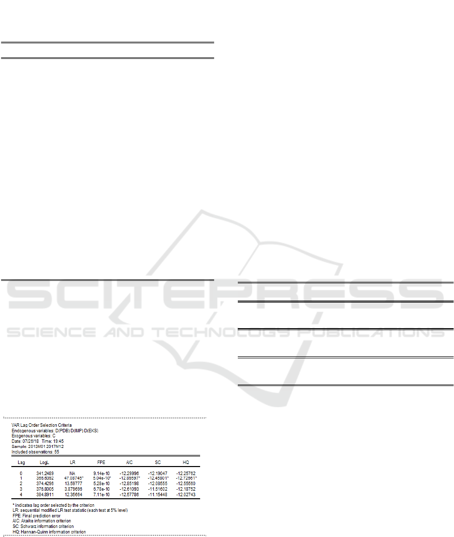
Table 3: Stability Test Lag Specification

According to the stability test, we can conclude

that VAR estimation that is used to analyze IRF and

VD is stable. Stability test results show that GDP

model is stable up to 9 (nine) maximum lag due to the

number of modulus value <1 or closer to 1, accounted

for 0.986964. Therefore, the conclusion is that the

data condition to all variables are stable

Table 4: Optimum Lag Criterion

Optimum lag test is important to remove auto-

correalation in VAR system. Therefore, by using

optimum lag, it will prevent the reappeared of

autocorrelation problem. Lag optimum determination

employs in this study referred to the shortest lag by

using Akaike Information Criterion (AIC). Pursuant

to GDP model, the lag optimum was at lag 1, so the

model can be analyzed to the next level. Similarly,

referred to other criteria such as LR FPE and HQ,

optimum lag was at lag 1. So, the final conclusion is

GDP model can be analyzed to the next step.

4.3 Granger Causality Test

Granger causality test is used to identify whether two

variables have causality relationship or parallel

relationship. Similarly, whether one variable

significantly has causality relationship to other

variables, this due to every single variable has an

opportunity to be endogenous variables or exogenous

variables. Bivariate causality test in this model

employs VAR pair-wise Granger causality test with

5% significant level. The Granger causality test result

is shown trough the following table.

Table 5: Optimum Lag Criterion

Granger causality test concludes that export

variables statistically insignificant affect to the GDP

(0.1426 > 0.05 this means that hypothesis 0 is

accepted, where there is no influence), similarly,

GDP also statistically insignificant affect to the

export (0.2631 > 0.05 this means that hypothesis 0 is

accepted, where there is no influence). Therefore, we

can conclude that there is no any causality to both

variables export and GDP.

Import variables statistically insignificant affect

to the GDP (0.1067 > 0.05 this means that hypothesis

0 is accepted, where there is no influence), similarly,

GDP also statistically insignificant affect to the

import (0.2692 > 0.05 this means that hypothesis 0 is

accepted, where there is no influence). Therefore, we

can conclude that there is no any causality to both

variables import and GDP.

Roots of Characteristic Polynomial

Endogenous variables: D(PDB) D(IMP) D(EKS)

Exogenous variables: C

Lag specification: 1 9

Date: 07/26/18 Tim e: 19:42

Root Modulus

-0.975034 + 0.152991i 0.986964

-0.975034 - 0.152991i 0.986964

-0.820279 - 0.542757i 0.983586

-0.820279 + 0.542757i 0.983586

-0.898787 + 0.379590i 0.975657

-0.898787 - 0.379590i 0.975657

-0.529881 + 0.807612i 0.965925

-0.529881 - 0.807612i 0.965925

0.207891 + 0.942804i 0.965452

0.207891 - 0.942804i 0.965452

0.458873 - 0.842485i 0.959346

0.458873 + 0.842485i 0.959346

-0.023307 - 0.957276i 0.957560

-0.023307 + 0.957276i 0.957560

-0.404443 - 0.858555i 0.949047

-0.404443 + 0.858555i 0.949047

0.919279 + 0.146570i 0.930890

0.919279 - 0.146570i 0.930890

0.640292 - 0.635954i 0.902448

0.640292 + 0.635954i 0.902448

0.748442 + 0.324116i 0.815608

0.748442 - 0.324116i 0.815608

-0.256055 - 0.713403i 0.757963

-0.256055 + 0.713403i 0.757963

0.422358 + 0.341532i 0.543167

0.422358 - 0.341532i 0.543167

-0.258676 0.258676

No root lies outs ide the unit circle.

VAR satisfies the stability condition.

Pairwise Granger Causality Tests

Date: 07/26/18 Time: 19:54

Sample: 2013M01 2017M12

Lags: 2

Null Hypothesis: Obs F-Statistic Prob.

IMP does not Granger Cause PDB 58 2.33515 0.1067

PDB does not Granger Cause IMP 1.34526 0.2692

EKS does not Granger Cause PDB 58 2.02093 0.1426

PDB does not Granger Cause EKS 1.36924 0.2631

EKS does not Granger Cause IMP 58 1.33607 0.2716

IMP does not Granger Cause EKS 0.16731 0.8464

The Role of International Trade to Economic Growth: The Case of Indonesia

2171

Import variables statistically insignificant affect

to the export (0.8464 > 0.05 this means that

hypothesis 0 is accepted, where there is no influence),

similarly, export also statistically insignificant affect

to the import (0.2716 > 0.05 this means that

hypothesis 0 is accepted, where there is no influence).

Therefore, we can conclude that there is no any

causality to both variables import and export.

4.4 Co-integration Test

Non-stationer data phenomenon at level can

produce the relationship of long-term balancing or

generally called as co-integration. Co-integration test

using Johansen co-integration test is aimed to identify

the co-integration relationship among variables. The

result of this test will determine the analysis method

that will be used whether VAR first difference or

VECM (Vector Error Correction Model)

Table 6: Johansen Co-integration Test

Table 6 identifies that trace statistic value and

eigenvalue maximum at r=0 are greater than critical

value at 5% significant level. This means that co-

integration test indicates that among the movement of

export, import, and GDP have the stability

relationship and the similarity of long-term

movement. In another word, every single short term

period, all variables tend to adjust to reach long-term

equilibrium.

4.5 VECM Estimation Model

VECM estimation result shows the short term and

long term relationship among variables (import,

export, and GDP). In this estimation, GDP is being

dependent variabels while independent variabels are

import and export. VECM estimation result used to

analyze short term and long term effect of

independent variable toward dependent variabels.

according to the table 7, it is clearly showed that there

is no significant effect export to GDP as well as

import to GDP in the short term.

Table 7: VECM Summary Result in Short Term

Variables Coefficient T-statistic

CointEq1

D(PDB(-1))

D(PDB(-2))

D(IMP(-1))

D(IMP(-2))

D(EKS (-1))

D(EKS (-2))

Meanwhile, table 8 provides longterm

information the influence of import and export toward

GDP. The result show that none of them has

significant influence in the long term.

Table 8: VECM Summary Result in Long Term

Variables Coefficient T-statistic

IMP (-1) -1.965642 -4.41480

EKS (-1) 2.767045 5.08545

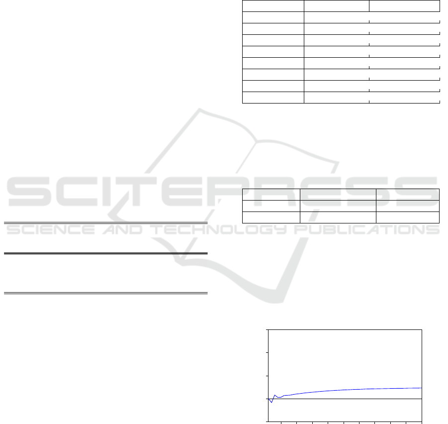
4.6 Impulse Response Function

Impulse response function describes the evolution of

the variable of GDP along a specified time horizon

after a shock in a given moment.

0.00092

[ 2.72704]

-0.45721

[-3.21668]

-0.29329

[-2.01217]

0.00754

[ 0.77692]

0.00297

[ 0.32424]

-0.01244

[-1.11248]

0.00348

[ 0.31076]

0.01352

[ 7.01490]

Date: 07/26/18 Time: 19:58

Sample (adjusted): 2013M04 2017M12

Included observations: 57 after adjustments

Trend assumption: Linear deterministic trend

Series: PDB IMP EKS

Lags interval (in first differences): 1 to 2

Unrestricted Cointegration Rank Test (Trace)

Hypothesized Trace 0.05

No. of CE(s) Eigenvalue Statistic Critical Value Prob.**

None * 0.266968 31.63824 29.79707 0.0303

At most 1 0.214944 13.93595 15.49471 0.0847

At most 2 0.002487 0.141932 3.841466 0.7064

Trace test indicates 1 cointegrating eqn(s) at the 0.05 level

* denotes rejection of the hypothesis at the 0.05 level

**MacKinnon-Haug-Michelis (1999) p-values

-.002

.000

.002

.004

.006

10 15 20 25 30 35 40 45 5

Response of PDB to EKS

ICRI 2018 - International Conference Recent Innovation

2172

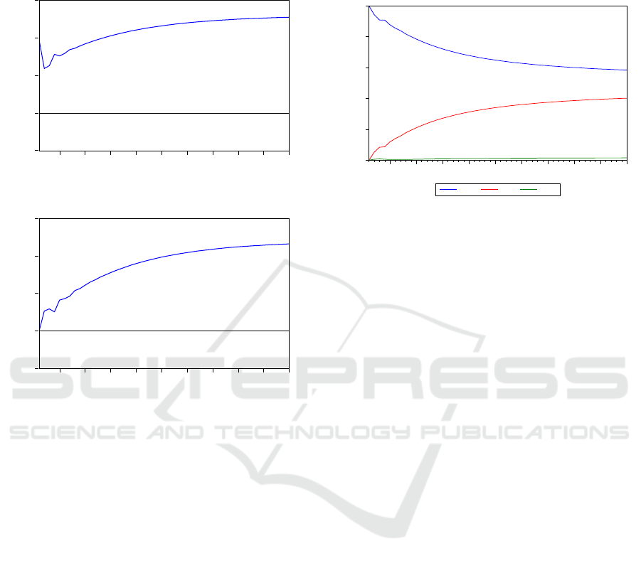
Figure 2: Impulse Response Function of Variables

Second graph of graph 2 shows the response of

GDP if it is shocked by import variable. GDP will

response the shock positively (+) strat from the first

period and fluctutaitve to the period 12 and remain

stable positively after period 14. The third graph

shows the response of GDP after shocked by export.

GDP respons negatively (-) strat from the second

period and start increasing to the positive trend after

period 3 and remain stable positive in the 10th period.

4.7 Variance Decomposition

Variance decomposition uses to determined a number

of contribution independent variables effect toward

dependent variable. Graph 3 describes the fulcutaion

of GDP difference, in the first period, GDP is greatly

affected by GDP itself. Import remain in second

priority after GDP start from the first period to period

of 50. From this graph, we can conclude that import

made the highest contribution toward GDP

respectively. In contrast, export was the least

significant part of GDP.

Figure 3: Variance Decomposition of GDP

4 CONCLUSIONS

From the previous briefly discussion regarding to the

export and import contribution toward economic

growth with VAR method, the conclusions of this

study is described as follow:

1. According to the impulse response function

analysis of the GDP model, it shows that GDP

will response negatively in short term and

positively stable in the long term in period of 15

due to the shocked of export.

2. According to the impulse response function

analysis of the GDP model, it shows that GDP

will response positively in short term and

positively stable in the long term in period of 20

due to the shocked of import.

There are various areas that can be improved from

current study for stakeholders and also further future

studies, which could include:

1. Overall, the largest contribution of GDP is highly

dependent on the government policy. If the

changes of economic conditions is not

appropriate to the previous forecasting, therefore

the government policy also must be changed so

the relationship as appeared as well as the

existing theory.

2. In consonance with plethora theories that there are

some macro economic variables affected to the

economic growth. This study is specifically using

export and import variables to determine its effect

toward economic growth, both short term and

long term. The author suggest for further study to

insert more variables such as inflation, exchange

rate, etc as intended to previous empirical studies.

Another main variable from Islamic financial

-.002

.000

.002

.004

.006

10 15 20 25 30 35 40 45 5

Response of PDB to PDB

-.002

.000

.002

.004

.006

10 15 20 25 30 35 40 45 5

Response of PDB to IMP

Response to Cholesky One S.D. Innovations

100

5 10 15 20 25 30 35 40 45 50

PDB IMP EKS

Variance Decomposition of PDB

The Role of International Trade to Economic Growth: The Case of Indonesia

2173

variables may be inserted such as asset and

financing of Islamic bank.

3. For further research is suggested to separate

research period into two main periods, before

crisis and after crisis (pre crisis and post crisis).

It is expected to have a briefly described of real

economic condition and throw over of good or

bad economic condition..

REFERENCES

Adeleye, J.O., Adeteye, O.S., & Adewuyi, M.O. (2015).

Impact of International Trade on Economic Growth in

Nigeria (1988-2012). International Journal of Financial

Research Vol 6, No 3.

Akanni, O.P. (2007). Oil Wealth and Economic Growth in

Oil Exporting Countries.AERC Research Oaoer, 170.

Ascarya. (2009).The Determinant of Inflation Under Dual

Monetary System in Indonesia. Center of Education

and Central Banking Studies, Bank Indonesia.

Ascarya., Soekarno, M., & Arianti, D. (2008).Dampak

Suku Bunga Kebijakan Terhadap Suku Bunga

Perbankan Indonesia dan Perbandingannya Dengan

Negara Lain.Center of Education and Central Banking

Studies, Bank Indonesia.

Boediono. (1999). Teori Pertumbuhan Ekonomi.

Yogyakarta: BPFE.

Gujarati, D. (2003). Ekonometrik Dasar. Terjemahan Oleh

Sumarno Zain. Jakarta: Erlangga.

Hashim, K., & Masih, M. (2014). What Causes Economic

Growth in Malaysia: Exports or Imports?.Munich

Personal RePEc Archive Paper No. 62366.

Hye, Q.M.A. (2012). Exports, Imports and Economic

Growth in China: An ARDL Analysis. Journal of

Chinese Economics and Foreign Trade Studies, Vol. 5

No. 1, pp 42-55.

Jhingan, M.L. (2005). The Economics of Development and

Planning.Vrinda Publication.

Kravis, I.B., Heston, A., and Summers, R. (1982). World

Product and Income: International Comparisons of Real

Gross Product. London: the Johns Hopkins University

Press.

Mazumdar, J. (2002). Imported Machinery and Growth in

LDCs. Journal of Development Economics. 65. pp 209-

224.

Rivai.M. (2006). “Pengaruh Ekspor, Impor dan Investasi

terhadap Pertumbuhan Ekonomi di Kalimantan Timur”.

Program Magister Ilmu Ekonomi Fakultas Ekonomi,

Universitas Mulawarman Samarinda.

Roshan, S.A. (2007). Export Linkage to Economic Growth:

Evidence from Iran. International Journal of

Development, Vol. 6, No.1, pp 38-49.

Seyoum, B. (2009). Export-Import Theory, Practices, and

Procedures: Second Edition. London: The Haworth

Press.

Shahbaz, M. & Rahman, M.M. (2014).Export, Financial

Development and Economic Growth in

Pakistan.International Journal of Development, Vol.

13, No. 2, pp 156-170.

Tanjung, H. & Devi, A. (2013).Metode Penelitian Ekonomi

Islam. Jakarta: PT Gramata Publishing.

Velnampy, T., & Achchuthan, S. (2013). Export, Import

and Economic Growth: Evidence from Sri Lanka.

Journal of Economics and Sustainable Development,

Vol 4, No 9.

Vohra.(2001). Exports and Economic Growth in

Developing Countries.Evidence from Time Series and

Cross-Section Data.Journal of Economic Development

and Cultural Change, 36, pp 51-72.

Won, Y., Hsiao, F.S.S.T, and Yang, D.Y. (2008). FDI

Inflows, Exports, and Economic Growth in First and

Second Generation ANIEs: Panel Data Causality

Analyses. KIEP Working Paper 08-02.

ICRI 2018 - International Conference Recent Innovation

2174