Tidal Effect on Sea Water Intake of Power Plant using CFD Model

Puspa Devita Mahdika Putri

and Suntoyo

Department of Ocean Engineering, Faculty of Marine Technology, Institut Teknologi Sepuluh Nopember (ITS),

Surabaya, 60111, Indonesia

Keywords: Computational Fluid Dynamics, Intake Channel, Turbulence, Vortex.

Abstract: To develop the capacity of electricity production in Indonesia, supporting infrastructure such as water intake

channel is necessary. By using water intake channel system, power companies can utilize seawater as a

cooling power plant. Water from the ocean is pumped into the cooling system to cool the generating engine.

In practice, the construction of intake channel often has a problem, especially in the pump section. One of the

most common problems is the vibration of the pumps caused by vortex flow. Based on research conducted by

Kim et al (2012), one of the causes of vortex flow is the speed difference. The free sea water surface has

several characteristics, one of which is sea tides. The tides can cause an acceleration that allows the vortex to

occur. For this reason, this paper perform numerical testing to determine how the effect of these tides on the

possibility of vortex flow in the intake channel. Moreover, the direction of vortices flow and shape that may

occur due to differences in elevation caused by tides is also examined.

1 INTRODUCTION

Grati Block 2 Power Plant with minimum net

dependable capacity of 150 MW is located in Desa

Lekok, Kabupaten Pasuruan, Indonesia. It utilize

circulating-water cooling systems that typically

require a number of large-scale, hydraulic pumps to

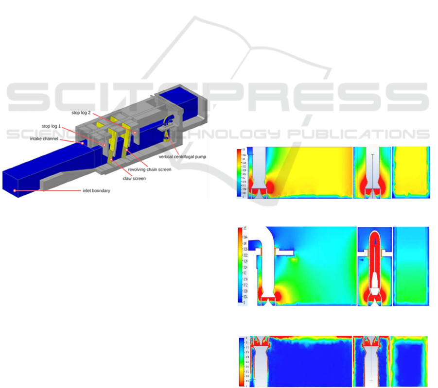
withdraw water from the sea. The system, as sketched

in Figure 1, comprises two pump-intake structures,

two stop logs, claw screen and revolving chain

screen. Warm waters enters each bay through a claw

screen and revolving chain screen, and is pumped into

a common discharge header.

Many of the large-scale vertical pumps installed

in power plants and various pumping stations have

experienced some sort of vibration, impeller damage

due to local cavitation, or loss of pumping efficiency

(Nakato, 1990). It caused primarily by nonuniform

pump-approach flow conditions in pump sumps that

known to produce prerotation and air-entraining free-

surface vortices. These nonuniformities in the intake

flow promote vibrations and excessive bearing loads.

Low pump intake submergence depths could result in

the formation of air-entraining free-surface vortices,

a phenomenon that significantly complicates the flow

Graduate Student

field and promotes cavitation (Constantinescu and

Patel, 1998).

Tides are the rise and fall of sea levels caused by

the combined effects of the gravitational forces

exerted by the moon, the sun, and the rotation of the

earth. Most places in the ocean usually experience

two high tides and two low tides each day, called

semidiurnal tide. Grati Pasuruan East Java sea waters

had mixed prevealing semi diurnal tide (Wijaya et al.,

2016). The difference of sea levels created by tides

can produce the difference velocity magnitude in

varies space. Thus it can impacts the flow conditions

inside the sea water intake. Fluid velocity becomes

faster when the sea levels is higher. It is considered

that the unstable flow develops the free surface vortex

(Kim et al, 2012).

Factors affecting the formation of vortices at

pump intakes have been known in general terms for

quite some time, there is no theoretical method for

predicting their ocuurence. Hence, it demands the full

power of modern computational fluid dynamics

(CFD) to solve the equations of motion and

turbulence models in domains that involve multiple

surfaces.

Putri, P. and Suntoyo, .

Tidal Effect on Sea Water Intake of Power Plant using CFD Model.

DOI: 10.5220/0009859102090211

In Proceedings of the 6th International Seminar on Ocean and Coastal Engineering, Environmental and Natural Disaster Management (ISOCEEN 2018), pages 209-211

ISBN: 978-989-758-455-8

209

2 METHOD AND NUMERICAL

SIMULATIONS

For perceiving and describing flow conditions in a

system, aside from physical observations, numerical

methods are also available. Flow fields can be

simulated by using Computational Fluid Dynamics

(CFD) techniques. To form the numerical model, the

first step is to construct a 3D model of the system in

computer environment. In CFD applications, the flow

environment is limited by boundary conditions to

simulate the surrounding effects on the particular

investigation area. The steps of a problem solution in

using Autodesk CFD can be listed as follows :

 The flow domain is defined

 Boundary conditions are defined

 Simulation start is given

Three models with different water elevation was

simulated to describe the difference result caused by

tides. The first water elevation that used in this case

is mean sea level (MSL) and the lowest low water

level (LLWL). For MSL, the water elevation is 6.67

m from bottom of the intake channel and LLWL is -

2.0 m from MSL.

Figure 1: Design of Intake Channel of Grati Power Plant.

2.1 Boundary Conditions

Boundary conditions have important role to create

similar flow conditions with the physical system.

There are three kind of boundary conditions used for

this design. The first boundary conditions is intake

boundary that placed in the inlet of the channel. The

intake boundary is defined with flowrate 50,000 m

and water temperature 30

C. Then, all region of wall

and screen was defined as slip/symetry boundary

condition. Rotating region with with a speed of 424

RPM also set for pump sump area. For the outlet

boundary, specified pressure 0 Pa boundary condition

was set.

2.2 Turbulence Model

In computation of turbulent flows, various turbulence

model options are avilable to solve Navier Stokes

equations. Prandtl mixing length, one equation

turbulent energy model, two equation (k-) model,

two equation (k-) model, Renormalized Group

Model (RNG) and Large Eddy simulation model are

possible options. In this case, the flow in this model

is constrained by a solid wall. The wall no-slip

condition ensures that, over some region of the wall

layer,viscous effects on the transport processes must

be large. The particular turbulence model such as the



model are not valid in the near-wall region as

shown in Suntoyo et al, 2008, Suntoyo and Tanaka,

2009, Suntoyo et al., 2016 where viscous effects are

dominant. Thus, the two equation (k-) SST

turbulence model works well in the wall-bounded

region but needs fine mesh close to the wall

(Andersson et al., 2012).

3 RESULT AND DISCUSSION

The result of CFD model using Autodesk CFD can be

analyzed by 2 variables, velocity magnitude and

vorticity magnitude. Two models with different sea

levels was simulated. The difference of velocity

magnitude and vorticity magnitude of two models

showed in Figure 2 - Figure 5.

Figure 2: Velocity Magnitude LLWL.

Figure 3: Velocity Magnitude HHWL.

Figure 4: Vorticity Magnitude LLWL.

ISOCEEN 2018 - 6th International Seminar on Ocean and Coastal Engineering, Environmental and Natural Disaster Management

210

Figure 5: Vorticity Magnitude HHWL.

Figure 2 and 3 show that the average velocity

magnitude near pump sumps were increased at lower

sea levels (LLWL). The average velocity at HHWL

and LLWL is about 1.36 m/s and 1.42 m/s. It was

observed that, due to the changed of sea levels, the

average velocity magnitude also changed. It was also

happened to vorticity at intake. Figure 4 and 5 show

that the average vorticity near pump sumps were

increased at smaller sea levels (LLWL). The average

vorticity at HHWL and LLWL is about 18.33 spin/s

and 19.1 spin/s. It was also observed that, due to the

changed of sea levels, the average vorticity also

changed.

4 CONCLUSIONS

According to the results from the CFD model, flow

velocity at LLWL is higher than HHWL. It means,

the lower sea level, the faster flow velocity. The

fastest flow velocity occured arround pump suctions,

at both HHWL and LLWL. Fluid vorticity also

become wider when the sea level is lower. It can

concluded that tides can impacts the flow

characteristics inside the intake and can produce the

difference of flow velocity that caused vortex flow.

REFERENCES

Andersson, B., Andersson, R., Hakansson, L., Mortensen,

M., Sudiyo, R., L. B. van Wachem, Hellstrom, 2012.

Computational Fluid Dynamics for Engineers.

Cambridge University Press. UK.

Kim, C.G., Choi Y.D., Choi, J.W., Lee, Y.H., 2012. A

Study on the Effectiveness of an Anti Vortex Device in

the Sump Model By Experiment and CFD. IOP

Conference Series Earth and Environmental Science

15(17): 1-11.

Constantinescu, G.S., Patel, V.C., 1998. Numerical Model

for Simulation of Pump-Intake Flow and Vortices.

Journal of Hydraulic Engineering. 124 (2): 123-134.

Nakato, T., 1990. A Hydraulic Model Study of the

Proposed Pump-Intake and Discharge Flume: Florida

Power Corporations Crystal River Helper Cooling-

Tower Project. IIHR Technical Report No. 339.

Suntoyo, Tanaka H., Sana A., 2008. Characteristics of

turbulent boundary layers over a rough bed under saw-

tooth waves and its application to sediment transport,

Coastal Engineering 55 (12): 1102-1112.

Suntoyo, Tanaka H., 2009. Effect of bed roughness on

turbulent boundary layer and net sediment transport

under asymmetric waves, Coastal Engineering 56 (9):

960-969.

Suntoyo, Fattah A.H., Fahmi M.Y., Rachman T., Tanaka

H., 2016 Bottom shear stress and bed load sediment

transport due to irregular wave motion, ARPN Journal

of Engineering and Applied Sciences 11(2): 825-829.

Wijaya, M. M., Suntoyo, Damerianne, H.A.. 2016. Bottom

shear stress and bed load sediment transport formula for

modeling the morphological change in the canal water

intake, ARPN Journal of Engineering and Applied

Sciences 11(4): 2723-2728.

Tidal Effect on Sea Water Intake of Power Plant using CFD Model

211