Hermite Interpolation by Piecewise Cubic
Trigonometric Spline with Shape Parameters
Said Hajji
1
, Abdellah Lamnii
2 a
, Boujemaa Danouj
1
and Mounir Lotfi
1
1
Univ. Hassan 1
st
, Laboratoire IMII, Faculty of Sciences and Technology, Settat, Morocco
2
Univ. Hassan 1
st
, Laboratoire MISI, Faculty of Sciences and Technology, Settat, Morocco
Keywords:
Hermite interpolation. Cubic trigonometric spline. Free-form curves and surfaces. Shape parameters.
Abstract:
In this paper, we are studing in depth a new cubic Hermite trigonometric spline interpolation method for
curves and surfaces with shape parameters. Based on this model of interpolation, we will give some examples
of free-form curves and surfaces, and analyse the effect of different shape parameters on the curve and surface
shape. We show that for λ = 1 −
√
2 and α =
1
4
the obtained cubic Hermite trigonometric curve or surface is
C
3
continuous. Finally, we will give an example of application, and we will discuss how the adjustment of the
shape parameters affects the shape of freeform surfaces.
1 INTRODUCTION
Nowadays, the worldwide trend of the mechanic
industry and more exactly the automotive industry
and aviation is marketed depend not only on func-
tional requirements, but also aesthetic ones. In ad-
dition, the continuous increase in energy charge is
pushing manufacturers to design product with aero-
dynamic,functional and aesthetic freeform shapes
(Savio et al., 2007). The design and prototyping stage
of free-form parts require the use of real model.
In the world of the automotive industry for exam-
ple, the initial design of a car wing is often done by
designers which concretize their concept by produc-
ing a model part. To begin or continue the produc-
tion process from these real models. They must be
transferred to a CAD system as a CAD model (Hajji
et al., 2018). Since this process aims to create a CAD
model from a physical part, (reverse engineering) and
obtain a good CAD model, the most important step is
the choice of the model to approximate the complex
surface from the set of points measured on the real
object.
The geometry of the curves and surfaces are
two theories which make it possible to describe the
complex forms. These complex shapes are usually
described using parametric surface representations
(Farin, 2001). The commonly used parametric sur-
faces are Ferguson et Coons Hermite, Spline, Bezier,
a
https://orcid.org/0000-0002-0538-8812
B-spline and B-spline surfaces, NURBS. Two excel-
lent references are (Farin, 2001), (Farin, 1999).
The paper is arranged as follows. Section 2, re-
calls the definition of cubic trigonometric polyno-
mial B-spline basis function (see (Liu et al., 2012)).
In Section 3, the cubic trigonometric polynomial B-
spline curve is given. Section 4 describes the con-
struction of cubic Hermite trigonometric spline inter-
polation, which is based on determining a set of cubic
Hermite trigonometric B-splines functions with shape
parameters. We will also give the definition of cubic
Hermite trigonometric spline curve associated at this
construction. Section 5 deals with the definition and
the smoothness of the interpolating surfaces. When
the shape parameters satisfy a simple condition, the
interpolating surface is C
3
. Finally, in order to illus-
trate our results, we will give in Section 6 some nu-
merical examples.
2 CUBIC TRIGONOMETRIC
POLYNOMIAL B-SPLINE BASIS
FUNCTION
In this section, we recall the definition and the inter-
esting properties of cubic trigonometric polynomial
B-spline Basis function, for more details see (Liu
et al., 2012).
Definition 1. For shape parameter, where −1 ≤λ ≤
1, t ∈ [0,
π
2
], the following four functions are defined
Hajji, S., Lamnii, A., Danouj, B. and Lotfi, M.
Hermite Interpolation by Piecewise Cubic Trigonometric Spline with Shape Parameters.
DOI: 10.5220/0009775302770283
In Proceedings of the 1st International Conference of Computer Science and Renewable Energies (ICCSRE 2018), pages 277-283
ISBN: 978-989-758-431-2
Copyright
c
 2020 by SCITEPRESS – Science and Technology Publications, Lda. All rights reserved
277

as the cubic trigonometric B-spline basis function
with a shape parameters λ:







B
0
(λ,t) = f (λ)(1 −sin(t))(1 −λ sin(t))
2
,
B
1
(λ,t) = f (λ)(1 + cos(t))(1 + λ cos(t))
2
,
B
2
(λ,t) = f (λ)(1 + sin(t))(1 + λ sin(t))
2
,
B
3
(λ,t) = f (λ)(1 −cos(t))(1 −λ cos(t))
2
,
(1)
where f (λ) =
1
2λ
2
+4λ+4
.
The cubic trigonometric polynomial B-spline Ba-
sis function possesses all the desirable properties of
classical polynomial B-splines, see (Liu et al., 2012).
• Nonnegative and Partition of unity: B
i
(λ,t) ≥
0, i = 0, 1, 2, 3 and
3
∑
i=0
B
i
(λ,t) = 1;
• Symmetry: B
0
(λ,t) = B
3
(λ,
π
2
−t), B
1
(λ,t) =
B
2
(λ,
π
2
−t);
• Monotony: where t ∈ [0,
π
2
], B
0
(λ,t) and B
3
(λ,t)
are monotonically decreasing for shape parameter
λ. B
1
(λ,t) and B
2
(λ,t) are monotonically increas-
ing for shape parameters λ, respectively.
3 CUBIC TRIGONOMETRIC
B-SPLINE CURVE WITH A
SHAPE PARAMETER
3.1 Definition and Properties
Definition 2. Given points V
i
(i = 0, 1, ··· , n + 1) in
R
2
or R
3
, −1 ≤ λ ≤ 1 and knots vectors U =
[u
1
, u
2
, ··· , u
n
]. For i = 1, ..., n −1, the i
th
trigono-
metric curve segment is given by:
V
i
(λ,t) :=
3
∑
j=0
V
i+ j−1
B
j
(λ,t), t ∈ [0,
π
2
]. (2)
In the same way, we can define the cubic trigonomet-
ric polynomial B-spline curve as follows :
V (λ,t) := V
i
(λ,
π
2
.
t−u
i
∆u
i
), t ∈ [u
i
, u
i+1
], (3)
where ∆u
i
= u
i+1
−u
i
, i = 1, 2, ··· , n −1, U is equidis-
tant knots vectors.
The cubic trigonometric B-spline curve (2) has the
following important geometric properties. For more
details see ((Liu et al., 2012)):
1. Terminal properties:















V (λ, 0) =
V
0
−2V
1
+V
2
2λ
2
+4λ+4
+V
1
,
V (λ,
π
2
) =
V
1
−2V
2
+V
3
2λ
2
+4λ+4
+V
2
,
V
0
(λ, 0) =
(2λ+1)(V
2
−V
0
)
2(λ(λ+2)+2)
,
V
0
(λ,
π
2
) =
(2λ+1)(V
3
−V
1
)
2(λ(λ+2)+2)
.
(4)
2. Symmetry: V
0
, ··· ,V
3
and V
3
, ··· ,V
0
define the
same trigonometric B-spline curve, i.e., V (λ,t) =
V (λ,
π
2
−t).
3. Geometric invariance: since the blending func-
tions have the properties of partition of unity, the
shape of these trigonometric B-spline curves is in-
dependent of the choice of coordinates.
4. Convex hull property: the blending functions have
the properties of nonnegativity and partition of
unity, as a consequence, the entire trigonometric
B-spline curve segment must lie inside the control
polygon spanned by V
0
, ··· ,V
3
.
5. Variation diminishing property.
3.2 Numerical Examples
By using the terminal properties we can construct an
open curve V (λ, t) interpolating V
0
and V
n+1
. In-
deed, it suffices to add four control points V
−2
=
V
−1
= V
0
and V
n+3
= V
n+2
= V
n+1
. For construct-
ing a trigonometric closed curve V (λ,t), we add four
control points V
−2
= V
n
, V
−1
= V
n+1
, V
n+2
= V
0
and
V
n+3
= V
1
. In Figure 1, the open and closed curves
are generated by altering the value of λ = 0.5: blue
color, λ = 0.8: red color and λ = 1: black color, U is
equidistant knots vectors. As λ increases, the curve is
closer to the control polygon.
(a) (b)
Figure 1: Effect of varying the shape parameter λ on the curve.
4 CUBIC HERMITE
TRIGONOMETRIC SPLINE
INTERPOLATION
4.1 Basis of the Cubic Hermite
Trigonometric Spline Interpolation
In analogy with the classical cubic polynomial Her-
mite function basis, we shall determine our trigono-
metric Hermite basis T B
α
0
(t), TB
α
1
(t), TB
α
2
(t) and
ICCSRE 2018 - International Conference of Computer Science and Renewable Energies
278

T B
α
3
(t) first by focusing on the interval [0,
π
2
] and im-
posing the four required boundary (endpoints) condi-
tions in each case, i.e.
T B
α
0
(0) = 0,T B
α
0
(
π
2
) = 0, T B
α(1)
0
(0) = −α
1
, T B
α(1)
0
(
π
2
) = 0,
T B
α
1
(0) = 1,T B
α
1
(
π
2
) = 0, T B
α(1)
1
(0) = 0, T B
α(1)
1
(
π
2
) = −α
2
,
T B
α
2
(0) = 0,T B
α
2
(
π
2
) = 1, T B
α(1)
2
(0) = α
1
, T B
α(1)
2
(
π
2
) = 0,
T B
α
3
(0) = 0,T B
α
3
(
π
2
) = 0, T B
α(1)
3
(0) = 0, T B
α(1)
3
(
π
2
) = α
2
.
The existence of the functions T B
α
0
, TB
α
1
,
T B
α
2
and T B
α
3
is guaranteed if we consider
hB
0
(λ,t), B
1
(λ,t), B
2
(λ,t), B
3
(λ,t)i as solutions space.
With a simple calculation we obtain the following ex-
pressions:



T B
α
0
(λ,t)
T B
α
1
(λ,t)
T B
α
2
(λ,t)
T B
α
3
(λ,t)



=



δ
0
δ
1
δ
2
δ
1
γ
1
γ
2
γ
1
γ
0
γ
0
γ
1
γ
2
γ
1
δ
1
δ
2
δ
1
δ
0






B
0
(λ,t)
B
1
(λ,t)
B
2
(λ,t)
B
3
(λ,t)



(5)
with
δ
0
=
α(2λ(λ+2)(λ(λ+2)+2)+1)
λ(λ+2)(2λ+1)
,
δ
1
=
−α(λ+1)
2
λ(λ+2)(2λ+1)
,
δ
2
=
α
λ(λ+2)(2λ+1)
,
γ
0
=
(λ+1)
2
(2λ+1)−α(2λ(λ+2)(λ(λ+2)+2)+1)
λ(λ+2)(2λ+1)
,
γ
1
=
α(λ+1)
2
−2λ−1
λ(λ+2)(2λ+1)
,
γ
2
=
(λ+1)
2
(2λ+1)−α
λ(λ+2)(2λ+1)
.
The four trigonometric Hermite basis functions
T B
α
i
, i = 0, ..., 3 are illustrated graphically in Figure
2. The trigonometric Hermite B-splines T B
α
i
, i =
0, ..., 3, has the following properties.
0 0.5 1 1.5
-0.1
0
0.1
0.2
0.3
0.4
0.5
0.6
0.7
0.8
(a) λ = 1 and α = 0.2.
0 0.5 1 1.5
-0.1
0
0.1
0.2
0.3
0.4
0.5
0.6
0.7
0.8
(b) λ = −1 and α = 0.7.
Figure 2: Trigonometric Hermite basis functions T B
α
i
, i = 0, ..., 3, with
various choice of λ and α.
Proposition 3. Let −1 ≤ λ ≤ 1. For any positive in-
teger α, the trigonometric functions TB
α
i
, i = 0, ··· , 3
satisfy the following properties:
• Partition of unity:
3
∑
i=0
T B
α
i
(λ,t) = 1, t ∈ [0,
π
2
].
• Symmetry:
T B
α
0
(λ,t) = TB
α
3
(λ,
π
2
−t), T B
α
1
(λ,t) = TB
α
2
(λ,
π
2
−t).
Proof. Indeed
3
∑
i=0
T B
α
i
(λ,t) = (δ
0
+ γ
1
+ γ
0
+ δ
1
)(B
0
(λ,t)+ B
3
(λ,t))
+ (δ
1
+ γ
2
+ γ
1
+ δ
2
)(B
1
(λ,t)+ B
2
(λ,t)).
On the other hand it is easy to verify that,
(δ
0
+ γ
1
+ γ
0
+ δ
1
) = 1 and (δ
1
+ γ
2
+ γ
1
+ δ
2
) = 1.
Then
3
∑
i=0
T B
α
i
(λ, .) = B
0
(λ, .) + B
1
(λ, .) + B
2
(λ, .) + B
3
(λ, .) = 1.
The symmetry stems from the symmetry of the basis
functions B
i
(λ,t) and the symmetry of lines 1 and 4
(respectively 2 and 3) of the system matrix (5).
4.2 Cubic Hermite Trigonometric Spline
Interpolation with Shape Parameters
Suppose that we are given four distinct points P
j
∈
R
2
, j = 0, ··· , 3. We are looking for a solution of the
trigonometric Hermite interpolation problem







T H
α
(λ, 0) = P
1
,
T H
α
(λ,
π
2
) = P
2
,
T H
(1)
α
(λ, 0) = α(P
2
−P
0
),
T H
(1)
α
(λ,
π
2
) = α(P
3
−P
1
).
(6)
where T H
α
(λ,t) : [0,
π
2
] −→ R
2
is a cubic paramet-
ric trigonometric curve, α is positive real and −1 ≤
λ ≤ 1. This situation is illustrated in Figure 3 (a). In
Figure 3 (b), we drew the cubic trigonometric Her-
mite spline curves associated with the four points
P
j
∈ R
2
, j = 0, ··· , 3, with various choice of shape
parameters λ and α.
Proposition 4. Let −1 ≤ λ ≤ 1 and α positive reel.
For any interpolation points P
j
, j = 0, ··· , 3, there ex-
ists a unique Hermite trigonometric spline interpola-
tion with shape parameters
T H
α
(λ,t) =
3
∑
j=0
P
j
T B
α
j
(λ,t), t ∈ [0,
π
2
],
satisfying the interpolation conditions (6).
4.3 Hermite Trigonometric Spline Curve
Definition 5. Given points P
i
(k = 0, 1, ···, n + 1) in
R
2
or R
3
, −1 ≤ λ ≤ 1, α > 0 and knots vectors U =
[u
1
, u
2
, ··· , u
n
]. For i = 1, ..., n −1, the i
th
Hermite
trigonometric spline curve segment is given by:
P
i
(λ,t) :=
3
∑
j=0
P
i+ j−1
T B
α
j
(λ,t), t ∈ [0,
π
2
]. (7)
In the same way, we can define the Hermite trigono-
metric spline curve made by all segments as:
P (λ, t) := P
i
(λ,
π
2
.
t−u
i
∆u
i
), t ∈ [u
i
, u
i+1
], (8)
Hermite Interpolation by Piecewise Cubic Trigonometric Spline with Shape Parameters
279

(a) (b)
Figure 3: (a) Cubic trigonometric Hermite spline curve created with four
control points. (b) Cubic trigonometric Hermite spline curves with various
choices of λ and α..
where ∆u
i
= u
i+1
−u
i
, i = 1, 2, ··· , n −1, U is equidis-
tant knots vectors.
Lemma 6. For Hermite trigonometric spline curve
(8), its continuity is as follows:
P
(k)
(λ, u
−
i
) =

∆u
i
∆u
i+1

k
P
(k)
(λ, u
+
i
), (9)
(a) when λ = 1 −
√
2 and α =
1
4
, k = 0, 1, 2, 3.
(b) when λ 6= 1 −
√
2 and ∀ α > 0, k = 0, 1, 3.
Proof.For (7), according to simple differential opera-
tion, until to third derivation, and more calculate, we
can gain:



























P
i−1
(λ,
π
2
) = P
i
(λ, 0) = P
i
P
(1)
i−1
(λ,
π
2
) = P
(1)
i
(λ, 0) = α(P
i+1
−P
i−1
)
P
(2)
i−1
(λ,
π
2
) =
α
(
2(λ+1)
2
P
i+1
+((λ−2)λ−1)(P
i−2
−P
i
)
)
2λ+1
+
2
(
−α(λ+1)
2
+2λ+1
)
P
i−1
−2(2λ+1)P
i
2λ+1
P
(2)
i
(λ, 0) =
α
(
2(λ+1)
2
(P
i−1
−P
i+1
)+((λ−2)λ−1)P
i+2
)
2λ+1
+
(α(1−(λ−2)λ)−4λ−2)P
i
+2(2λ+1)P
i+1
2λ+1
P
(3)
i−1
(λ,
π
2
) = P
(3)
i
(λ, 0) =
5
4
(P
i+1
−P
i−1
).
So that,
P
(k)
i−1
(λ,
π
2
) = P
(k)
i
(λ, 0), |λ| ≤ 1, α > 0, k = 0, 1, 3. (10)
Let u ∈ [u
i
, u
i+1
], t =
π
2
.
u−u
i
∆u
i
, then P
(k)
(λ, u) =

π
2
.
1
∆u
i

k
P
(k)
i
(λ,t).
Then
P
(k)
(λ, u
−
i
) =

π
2
.
1
∆u
i−1

k
P
(k)
i−1
(λ,
π
2
), (11)
P
(k)
(λ, u
+
i
) =

π
2
.
1
∆u
i

k
P
(k)
i−1
(λ, 0).
According to (10) and (11), the Lemma 6 holds. The
Lemma 6 shows that P (λ, u) is C
1
continuity if λ =
1 −
√
2 and α =
1
4
, is C
3
continuity.
In Figures 4 and 5, we give an examples of open
and close cubic trigonometric Hermite spline inter-
polant curves with various choice of λ and α. In the
case λ = 1 −
√
2, α =
1
4
the curve is is C
3
continuity,
on the other hand in the other cases we only have a is
C
1
continuity.
(a) λ = −0.1, α =
3
4
. (b) λ = 0.5, α =
1
2
. (c) λ = 1 −
√
2, α =
1
4
.
Figure 4: An open cubic trigonometric Hermite spline interpolant curves
with various choice of λ and α.
(a) λ = −0.1, α =
3
4
. (b) λ = 0.5, α =
1
2
. (c) λ = 1 −
√
2, α =
1
4
.
Figure 5: A close cubic trigonometric Hermite spline interpolant curves
with various choice of λ and α.
5 CUBIC TRIGONOMETRIC
HERMITE PARAMETRIC
SPLINE SURFACES
Similarly to the work done by Y. ZHU et al. (see
(Zhu et al., 2012)), we define trigonometric paramet-
ric spline surfaces as a tensor product. More precisely
we have the following definition.
Definition 7. Given (n + 2) ×(n + 2) interpolation
points P
i j
, knot vectors U = [u
1
, u
2
, ··· , u
n
] and α > 0.
For −1 ≤ λ ≤ 1, the trigonometric parametric spline
surface patch has the form :
S
i, j
(λ,t, s) :=
3
∑
k=0
3
∑
l=0
P
i+k−1, j+l−1
T B
α
k
(λ,t)TB
α
l
(λ, s),
(t, s) ∈ [0,
π
2
] ×[0,
π
2
].
Then the trigonometric parametric spline surface is
given by,
S (λ, t, s) := S
i, j
(λ,
π
2
.
t−u
i
∆u
i
,
π
2
.
s−u
j
∆u
j
), (12)
(t, s) ∈ [u
i
, u
i+1
] ×[u
j
, u
j+1
].
where ∆u
i
= u
i+1
−u
i
.
The surface S (λ, t, s) has the following interpola-
tion property.
ICCSRE 2018 - International Conference of Computer Science and Renewable Energies
280

Lemma 8. The (i, j)
th
bi-trigonometric Hermite
segment patch S
i, j
(u, v) verifies the following inter-
polating properties:
S
i, j
(λ, 0, 0) = S
i, j−1
(λ, 0,
π
2
)
= S
i−1, j
(λ,
π
2
, 0) = S
i−1, j−1
(λ,
π
2
,
π
2
) = P
i, j
,
∂
∂t
S
i, j
(λ, 0, 0) =
∂
∂t
S
i, j−1
(λ, 0,
π
2
)
=
∂
∂t
S
i−1, j
(λ,
π
2
, 0) =
∂
∂t
S
i−1, j−1
(λ,
π
2
,
π
2
)
= α (P
i+1, j
−P
i−1, j
),
∂
∂s
S
i, j
(λ, 0, 0) =
∂
∂s
S
i, j−1
(λ, 0,
π
2
)
=
∂
∂s
S
i−1, j
(λ,
π
2
, 0) =
∂
∂s
S
i−1, j−1
(λ,
π
2
,
π
2
)
= α (P
i, j+1
−P
i, j−1
),
∂
2
∂t∂s
S
i, j
(λ, 0, 0) =
∂
2
∂t∂s
S
i, j−1
(λ, 0,
π
2
)
=
∂
2
∂t∂s
S
i−1, j
(λ,
π
2
, 0) =
∂
2
∂t∂s
S
i−1, j−1
(λ,
π
2
,
π
2
)
= α
2
(P
i−1, j−1
−P
i−1, j+1
−P
i+1, j−1
+ P
i+1, j+1
),
∂
2
∂
2
t
S
i, j
(λ, 0, 0) =

−αλ
2
+2(α−2)λ+α−2

P
i, j
+2α(λ+1)
2
P
i−1, j
2λ+1
−
2

α(λ+1)
2
−2λ−1

P
i+1, j
+α((λ−2)λ−1)P
i+2, j
2λ+1
,
∂
2
∂
2
t
S
i, j−1
(λ, 0,
π
2
) =

−αλ
2
+2(α−2)λ+α−2

P
i, j
+2α(λ+1)
2
P
i−1, j
2λ+1
−
2

α(λ+1)
2
−2λ−1

P
i+1, j
+α((λ−2)λ−1)P
i+2, j
2λ+1
,
∂
2
∂
2
t
S
i−1, j
(λ,
π
2
, 0) =

−αλ
2
+2(α−2)λ+α−2

P
i, j
+2α(λ+1)
2
P
i+1, j
2λ+1
+
α((λ−2)λ−1)P
i−2, j
−2

α(λ+1)
2
−2λ−1

P
i−1, j
2λ+1
,
∂
2
∂
2
t
S
i−1, j−1
(λ,
π
2
,
π
2
) =

−αλ
2
+2(α−2)λ+α−2

P
i, j
+2α(λ+1)
2
P
i+1, j
2λ+1
+
α((λ−2)λ−1)P
i−2, j
−2

α(λ+1)
2
−2λ−1

P
i−1, j
2λ+1
,
∂
2
∂
2
s
S
i, j
(λ, 0, 0) =

−αλ
2
+2(α−2)λ+α−2

P
i, j
+2α(λ+1)
2
P
i, j−1
2λ+1
−
2

α(λ+1)
2
−2λ−1

P
i, j+1
+α((λ−2)λ−1)P
i, j+2
2λ+1
,
∂
2
∂
2
s
S
i, j−1
(λ, 0,
π
2
=

−αλ
2
+2(α−2)λ+α−2

P
i, j
+2α(λ+1)
2
P
i, j+1
2λ+1
+
α((λ−2)λ−1)P
i, j−2
−2

α(λ+1)
2
−2λ−1

P
i, j−1
2λ+1
,
∂
2
∂
2
s
S
i−1, j
(λ,
π
2
, 0) =

−αλ
2
+2(α−2)λ+α−2

P
i, j
+2α(λ+1)
2
P
i, j+1
2λ+1
+
α((λ−2)λ−1)P
i, j−2
−2

α(λ+1)
2
−2λ−1

P
i, j−1
2λ+1
,
∂
2
∂
2
s
S
i−1, j−1
(λ,
π
2
,
π
2
) =

−αλ
2
+2(α−2)λ+α−2

P
i, j
+2α(λ+1)
2
P
i, j+1
2λ+1
+
α((λ−2)λ−1)P
i, j−2
−2

α(λ+1)
2
−2λ−1

P
i, j−1
2λ+1
,
∂
3
∂
3
t
S
i, j
(λ, 0, 0) =
∂
3
∂
3
t
S
i, j−1
(λ, 0,
π
2
) =
∂
3
∂
3
t
S
i−1, j
(λ,
π
2
, 0)
=
∂
3
∂
3
t
S
i−1, j−1
(λ,
π
2
,
π
2
) = −
α

6λ
2
−2λ−1

(
P
i−1, j
−P
i+1, j
)
2λ+1
,
∂
3
∂
3
s
S
i, j
(λ, 0, 0) =
∂
3
∂
3
s
S
i, j−1
(λ, 0,
π
2
) =
∂
3
∂
3
s
S
i−1, j
(λ,
π
2
, 0)
=
∂
3
∂
3
s
S
i−1, j−1
(λ,
π
2
,
π
2
) = −
α

6λ
2
−2λ−1

(
P
i, j−1
−P
i, j+1
)
2λ+1
,
∂
3
∂
2
t∂s
S
i, j
(λ, 0, 0) =
∂
3
∂
2
t∂s
S
i, j−1
(λ, 0,
π
2
)
=
∂
3
∂
2
t∂s
S
i−1, j
(λ,
π
2
, 0) =
∂
3
∂
2
t∂s
S
i−1, j−1
(λ,
π
2
,
π
2
)
=

αλ
2
P
i, j−1
−αλ
2
P
i, j+1
+ 2αλ
2
P
i+1, j−1
−
2αλ
2
P
i+1, j+1
−αλ
2
P
i+2, j−1
+ αλ
2
P
i+2, j+1
−2αλP
i, j−1
+ 2αλP
i, j+1
+ 4αλP
i+1, j−1
−
4αλP
i+1, j+1
+ 2αλP
i+2, j−1
−2αλP
i+2, j+1
−2α(λ + 1)
2
P
i−1, j−1
+ 2α(λ + 1)
2
P
i−1, j+1
−
αP
i, j−1
+ αP
i, j+1
+ 2αP
i+1, j−1
−2αP
i+1, j+1
+αP
i+2, j−1
−αP
i+2, j+1
+ 4λP
i, j−1
−4λP
i, j+1
−4λP
i+1, j−1
+ 4λP
i+1, j+1
+ 2P
i, j−1
−2P
i, j+1
−2P
i+1, j−1
+ 2P
i+1, j+1

α
1+λ
,
∂
3
∂t∂
2
s
S
i, j
(λ, 0, 0) =
∂
3
∂t∂
2
s
S
i, j−1
(λ, 0,
π
2
)
=
∂
3
∂t∂
2
s
S
i−1, j
(λ,
π
2
, 0) =
∂
3
∂t∂
2
s
S
i−1, j−1
(λ,
π
2
,
π
2
)
=

2αλ
2
P
i−1, j+1
−αλ
2
P
i−1, j+2
+ 2αλ
2
P
i+1, j−1
−
αλ
2
P
i+1, j
−2αλ
2
P
i+1, j+1
+ 4αλP
i−1, j+1
2αλP
i−1, j+2
+ 4αλP
i+1, j−1
+ 2αλP
i+1, j
−
+4αλP
i+1, j+1
−2α(λ + 1)
2
P
i−1, j−1
+ (α(λ −2)
4λ + 2)P
i−1, j
+ α((λ −2)λ −1)P
i+1, j+2
+αP
i−1, j+2
+ 2αP
i+1, j−1
+ αP
i+1, j
−2αP
i+1, j+1
−4λP
i−1, j+1
−4λP
i+1, j
+ 4λP
i+1, j+1
−
2(P
i−1, j+1
+ P
i+1, j
−P
i+1, j+1
)

α
1+λ
.
Figure 6(a), illustrate the data used to determine
the bi-trigonometric Hermite segment patch S
i, j
(u, v).
Hermite Interpolation by Piecewise Cubic Trigonometric Spline with Shape Parameters
281

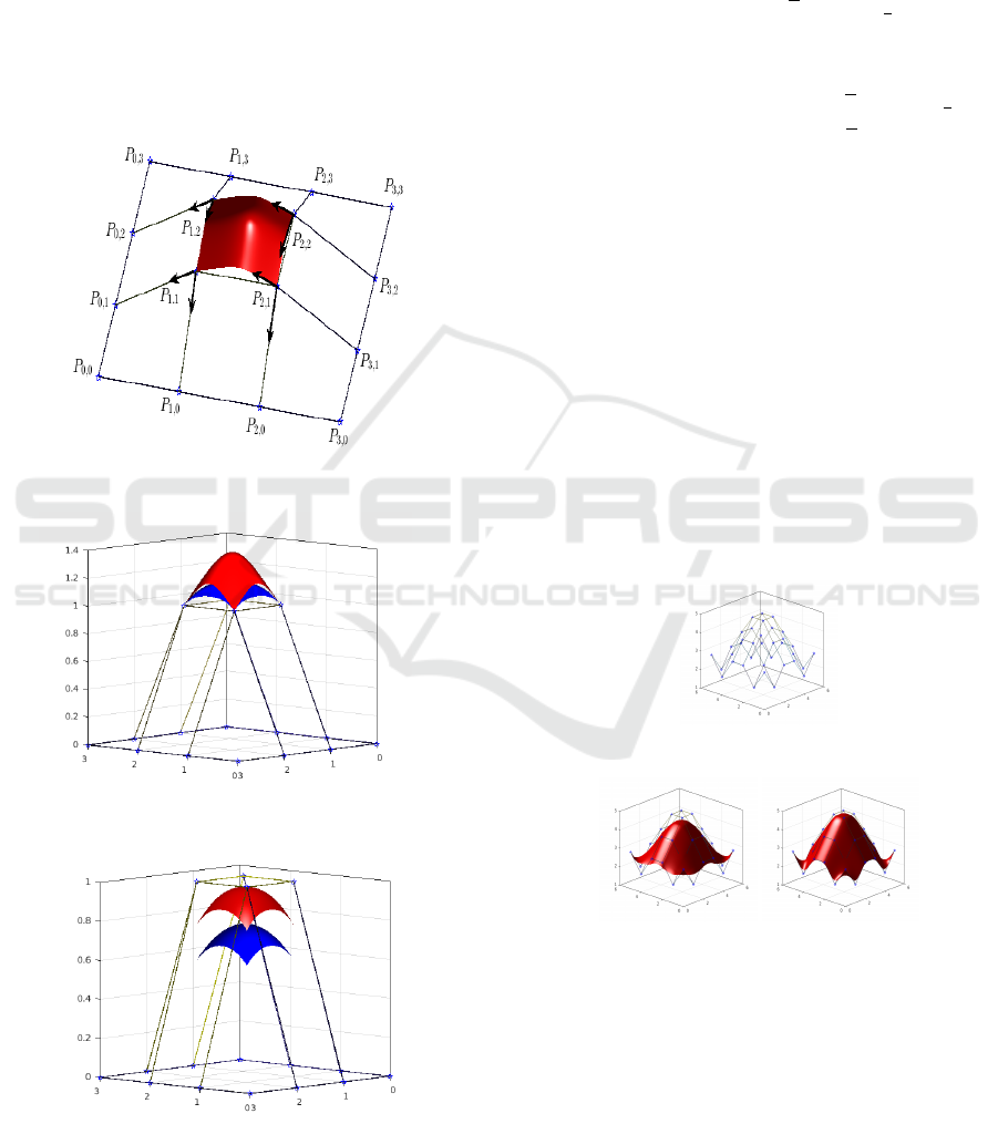
Figure 6(b), shows bi-trigonometric Hermite surface
patch with different parameters: λ = −1 and α = 0.2
(red) and λ = 1 and α = 0.2 (blue). Figure 6(c), shows
bicubic trigonometric surface patch using the defini-
tion of H. Liu et al. (see (Liu et al., 2012)) with dif-
ferent parameters: λ = 1 (red) and λ = 0 (blue).
(a)
(b)
(c)
Figure 6: Bicubic trigonometric and bi-trigonometric Her-
mite B-spline surface patch with different parameters.
The surface S (λ, t, s) resulting of union of bi-
trigonometric Hermite segments patch S
i, j
(λ,t, s) will
have continuous first order derivatives and continuous
crossed derivative. In the cubic trigonometric Her-
mite surfaces S(λ, t, s), C
1
continuity between two
surfaces is a direct consequence of the construction
of this interpolant. So much so the C
3
continuity is
forced by imposing λ = 1 −
√
2 and α =
1
4
. More pre-
cisely, we have the following result.
Proposition 9. The surface (12) is
(a) C
3
-continuous, when λ = 1 −
√
2 and α =
1
4
.
(b) C
1
-continuous, when λ 6= 1 −
√
2 and ∀ α > 0.
6 EXAMPLES FOR
APPLICATION
In order to justify the accuracy and efficiency of
our presented cubic trigonometric Hermite interpola-
tion we consider some graphical examples. For con-
structing a bicubic trigonometric or bi-trigonometric
Hermite B-spline surface patch interpolating the four
edges of the resulting surface, we add four col-
umn vectors of control points (P
i,−2
= P
i,−1
= P
i,0
and P
i,n+3
= P
i,n+2
= P
i,n+1
, i = 0, 1, ···, n + 1) and
four row vectors(P
−2, j
= P
−1, j
= P
0, j
and P
n+3, j
=
P
n+2, j
= P
n+1, j
, j = 0, 1, ···, n + 1).
(a) Control Points.
(b) λ = −0.1 (c) λ = 1
Figure 7: Bicubic B-spline surface patch with different parameters.
ACKNOWLEDGEMENTS
The authors are grateful to the University Hassan 1
st
for their support.
ICCSRE 2018 - International Conference of Computer Science and Renewable Energies
282

(a) λ = 1 −
√
2 and α =
1
4
.
(b) λ = 0.3 and α = 0.4. (c) λ = 1 and α = 0.45.
Figure 8: Bicubic B-spline surface patch with different parameters.
(a) Control Points.
(b) λ = 0 (c) λ = 1
Figure 9: Bicubic B-spline surface patch with different parameters.
(a) λ = 1 −
√
2 and α =
1
4
.
(b) λ = 0.3 and α = 0.4. (c) λ = 1 and α = 0.45.
Figure 10: Bicubic B-spline surface patch with different parameters.
(a) λ = 1.
(b) λ = 0.3 and α = 0.4. (c) λ = 1 and α = 0.45.
Figure 11: Bicubic B-spline surface patch with different parameters.
REFERENCES
Farin, G. (1999). Nurbs: From projective geometry to prac-
tical use,. In 2nd edition, Wellesley, MA, AK Peters.
Farin, G. (2001). Curves and surfaces for cagd. In A Prac-
tical Guide 5th Edition. CADG.
Hajji, S., Danouj, B., and Lamnii, A. (2018). Uat b-splines
of order 4 for reconstructing the curves and surfaces.
In Applied Mathematical Sciences,. HIKARI Ltd.
Liu, H., Li, L., Zhang, D., and Wang, H. (2012). Cubic
trigonometric polynomial b-spline curves and surfaces
with shape parameter. In Journal of Information &
Computational Science.
Savio, E., Chiffre, L. D., and Schmitt, R. (2007). Metrology
of freeform shaped parts. In CIRP Annals.
Zhu, Y., Han, X., and Han, J. (2012). Quartic trigonomet-
ric bezier curves and shape preserving interpolation
curves,. In Journal of Computational Information Sys-
tems.
Hermite Interpolation by Piecewise Cubic Trigonometric Spline with Shape Parameters
283