Propagation of Reaction Front in Porous Media under Natural
Convection
Khalfi Oussama
1
, Karam Allali
1
1
Department of Mathematics, Faculty of Science and Technology, University Hassan II, PO-Box 146, Mohammedia,
Keywords:
Boussinesq approximation, convection, Darcy law, linear stability analysis, Vadasz number.
Abstract:
This paper examines the influence of convective instability on the reaction front propagation in porous media.
The model includes heat and concentration equations and motion equations under Boussinesq approximation.
The non-stationary Darcy equation is adopted and the fluid is supposed to be incompressible. Numerical
results are performed via the dispersion relation. The simulations show that the propogating reaction front
loses stability as Vadasz number increase, it shows also more stability is gained when Zeldovich number
increased.
1 INTRODUCTION
The reaction front propagation in porous media
presents much important interest in many techno-
logical and scientifical fields like biology, ecology,
groundwater, hydrology, oil recovery to name just
a few (see for instance (Murphy, 2000; Linninger,
2008; Stevens, 2009; Nield, 2006; Gaikwad, 2015;
Faradonbeh, 2015); and references therein). In or-
der to describe the flow dynamics in porous media,
one can use the quasi-stationary or the non-stationary
Darcy equation combined to reaction-diffusion equa-
tions. In porous media, the reaction front propaga-
tion under convective effect has been studied by (Al-
lali et al., 2007; Allali, 2014); the authors have used
the reaction-diffusion equations coupled with a quasi-
stationary Darcy equation. In an other work, the au-
thors in (Khalfi. O, 2016) use non-sationary Darcy
equation and they study the influence of the reaction
front by depicting the evolution of Zeldovich num-
ber versus wave number and versus Vadasz number
highlight the influence of Vasdasz number on convec-
tive instability. In this work, an extension of this last
study will be done to the same model wich describ the
reaction front propagation with non-stationary Darcy
equation; that model will be considered and deliv-
red to linear stability analysis. For this objectif, the
porous media is considerd to be filled by an incom-
pressible fluid, morover the reaction front propagates
in opposite sense of gravity. To perform the linear
stability analysis, the Zeldovich-Frank-Kamenetskii
method is used. The interface problem is obtained
and the stability boundary is found from the derived
dispersion relation.
This paper is organized as follows. The next sec-
tion will be devoted to the governing equations, fol-
lowed in Section 3 by the linear stability analysis. Nu-
merical simulations are performed in Section 4. last
section concludes the work.
2 GOVERNING EQUATIONS
The propagating reaction front in porous media
can be modelled as follows:
∂T
∂t
+ v.∇T = κ∆T + qK(T )φ(α), (1)
∂α
∂t
+ v.∇α = d∆α + K(T)φ(α), (2)
∂v
∂t
+
µ
K
v + ∇p = gβρ(T −T
0
)γ, (3)
∇.v = 0, (4)
under the following boundary conditions:
T = T
i
, α = 1 and v = 0 when y →+∞, (5)
T = T
b
, α = 0 and v = 0 when y →−∞, (6)
here β denotes the coefficient of thermal expan-
sion, µ the viscosity, K
p
the permeability of the porous
media, γ the upward unit vector in the vertical direc-
tion, T the temperature, α the depth of conversion, v
Oussama, K. and Allali, K.
Propagation of Reaction Front in Porous Media under Natural Convection.
DOI: 10.5220/0009774101670174
In Proceedings of the 1st International Conference of Computer Science and Renewable Energies (ICCSRE 2018), pages 167-174
ISBN: 978-989-758-431-2
Copyright
c
 2020 by SCITEPRESS – Science and Technology Publications, Lda. All rights reserved
167

the velocity, p the pressure, κ the coefficient of ther-
mal diffusivity, d the diffusion coefficient, q the adi-
abatic heat release, g the gravity acceleration, ρ the
density. Finally, ∇ and ∆ denote the standard differ-
ential operators,
in addition T
0
is the mean value of the tempera-
ture, T
i
is an initial temperature while T
b
is the tem-
perature of the reacted mixture given by T
b
= T
i
+ q.
The function K(T )φ(α) is the reaction rate where the
temperature dependence is given by the Arrhenius ex-
ponential:
K(T) = k
0
exp

−
E
R
0
T

, (7)
E means the activation energy, R
0
the universal
gas constant and k
0
the pre-exponential factor.
2.1 The Dimensionless Model
For the dimensionless model, we introduce the spa-
tial variables y
0
=
yc
κ
, x
0
=
xc
κ
, time t
0
=
tc
2
κ
, velocity
v =
v
c
and the pressure p
0
=
pµκ
K
are introduced. De-
noting θ =
T −T
b
q
and omitting the primes of the new
variables, the model becomes:
∂θ
∂t
+ v.∇θ = ∆θ +W (θ)φ(α), (8)
∂α
∂t
+ v.∇α = Λ∆α +W (θ)φ(α), (9)
1
V
a
∂v
∂t
+ v + ∇p = R
p
(θ + θ
0
)γ, (10)
∇.v = 0, (11)
which is supllemented by the following conditions
in infinity:
θ = −1, α = 1 and v = 0 when y → +∞, (12)
θ = 0, α = 0 and v = 0 when y → −∞. (13)
Here W(θ) = Z exp

θ
Z
−1
+ δθ

, where Z =
qE
R
0
T
2
b
is
the Zeldovich number, δ =
R
0
T
b
E
,
θ
0
=
T
b
−T
0
q
, Λ =
d
κ
is the inverse of Lewis num-
ber, R
p
=
K
p
c
2
P
2
r
R
µ
2
where R is the Rayleigh number
defined by R =
gβqκ
2
µc
3
, P
r
is the Prandtl number de-
fined by P
r
=
µ
κ
, V
a
=
κµ
K
p
c
2
is the Vadasz number

called also Darcy-Prandtl number; V
a
wich is given
by V
a
=
D
a
P
r
, where D
a
is the Darcy number defined by
D
a
=
c
2
K
p
κ
2

. In what follows, Λ = 0 will be consid-
ered, wich corresponds to liquid mixture.
3 LINEAR STABILITY ANALYSIS
3.1 Approximation of Infinitely Narrow
Reaction Zone
By using an analytical study which reduces the prob-
lem (8)-(13) to a singular perturbation one, where
the reaction zone is assumed to be narrow (which is
named the reaction front), the linear stability analysis
is performed. The reaction source term is neglected
ahead of the reaction front (because the temperature
is not sufficiently high) and behind the reaction front
(since in this region there are no fresh reactant left).
This approach, called Zeldovich-Frank-Kamenetskii
approximation, leads to an interface problem by ap-
plying a formal asymptotic analysis for large Zel-
dovich number. In other words, for this asymptotic
analysis treatment, let considers ε =
1
Z
as a small pa-
rameter. And let assum by ζ(t, x) the location of the
reaction zone, and consider the new independent vari-
able is
y
1
= y −ζ(t,x). (14)
Taking into account those new statements, the new
functions θ
1
, α
1
, v
1
, p
1
can be written as:
θ(t,x,y) = θ
1
(t,x,y
1
), α(t,x,y) = α
1
(t,x,y
1
),
v(t,x,y) = v
1
(t,x,y
1
), p(t,x,y) = p
1
(t,x,y
1
).
(15)
By the way, the equations will be re-written in the fol-
lowing form (the index 1 for the dependent variables
is omitted):
∂θ
∂t
−
∂θ
∂y
1
∂ζ
∂t
+ v ·
e
∇θ =
e
∆θ +W (θ)φ(α), (16)
∂α
∂t
−
∂α
∂y
1
∂ζ
∂t
+ v ·
e
∇α = W (θ)φ(α), (17)
1
V
a
(
∂v
∂t
−
∂v
∂y
1
∂ζ
∂t
) + v +
˜
∇p = R
p
(θ + θ
0
)γ, (18)
∂v
x
∂x
−
∂v
x
∂y
1
∂ζ
∂x
+
∂v
y
∂y
1
= 0, (19)
where
e
∆ =
∂
2
∂x
2
+
∂
2
∂y
2
1
−2
∂ζ
∂x
∂
2
∂x∂y
1
+

∂ζ
∂x

2
∂
2
∂y
2
1
−
∂
2
ζ
∂x
2
∂
∂y
1
,
(20)
ICCSRE 2018 - International Conference of Computer Science and Renewable Energies
168

e
∇ =

∂
∂x
−
∂ζ
∂x
∂
∂y
1
,
∂
∂y
1

. (21)
To find the jump conditions approximation and so-
lution of the interface problem, the matched asymp-
totic expansions method is used. To this aim, the outer
solution of the problem is sought in the form:
θ = θ
˘
0
+ εθ
˘
1
+ ..., α = α
˘
0
+ εα
˘
1
+ ...,
v = v
˘
0
+ εv
˘
1
+ ..., p = p
˘
0
+ εp
˘
1
+ ....
(22)
For the inner solution, the stretching coordinate
η = y
1
/ε is introduced and the inner solution is sought
in the following form:
θ = ε
˜
θ
˘
1
+ ..., α =
˜
α
˘
0
+ ε
˜
α
˘
1
+ ...,
v =
˜
v
˘
0
+ ε
˜
v
˘
1
+ ..., p = ˜p
˘
0
+ ε ˜p
˘
1
+ ...,
ζ =
˜
ζ
˘
0
+ ε
˜
ζ
˘
1
+ ....
(23)
Substituting these expansions into (16)-(19),
it follows:
order ε
−1

1 +

∂
˜
ζ
˘
0
∂x

2

∂
2
˜
θ
˘
1
∂η
2
+exp

˜
θ
˘
1
1 + δ
˜
θ
˘
1

φ(
˜
α
˘
0
) = 0,
(24)
−
∂
˜
α
˘
0
∂η
∂
˜
ζ
˘
0
∂t
−
∂
˜
α
˘
0
∂η

˜v
˘
0
x
∂
˜
ζ
˘
0
∂x
− ˜v
˘
0
y

= exp

˜
θ
˘
1
1 + δ
˜
θ
˘
1

φ(
˜
α
˘
0
), (25)
−
1
V
a
∂ ˜v
˘
0
x
∂η
∂
˜
ζ
˘
0
∂t
−
∂ ˜p
˘
0
∂η
∂
˜
ζ
˘
0
∂x
= 0, (26)
−
1
V
a
∂ ˜v
˘
0
y
∂η
∂
˜
ζ
˘
0
∂t
−
∂ ˜p
˘
0
∂η
= 0, (27)
−
∂ ˜v
˘
0
x
∂η
∂
˜
ζ
˘
0
∂x
+
∂ ˜v
˘
0
y
∂η
= 0, (28)
order ε
0
1
V
a

∂v
˘
0
x
∂t
−
∂v
˘
1
x
∂η
∂ζ
˘
0
∂t
−
∂ζ
˘
1
∂t
∂v
˘
0
x
∂η

+
∂p
˘
0
∂x
−
∂p
˘
0
∂η
∂ζ
˘
1
∂x
−
∂p
˘
1
∂η
∂ζ
˘
0
∂x
+ v
˘
0
x
= R
p
θ
0
, (29)
1
V
a

∂v
˘
0
y
∂t
−
∂v
˘
1
y
∂η
∂ζ
˘
0
∂t
−
∂ζ
˘
1
∂t
∂v
˘
0
y
∂η

+
∂p
˘
1
∂η
+ v
˘
0
y
= R
p
θ
0
,
(30)
order ε
1
1
V
a

∂ ˜v
˘
0
x
∂t
−
∂ ˜v
˘
0
x
∂η
∂
˜
ζ
˘
2
∂t
−
∂ζ
˘
1
∂η
∂ ˜v
˘
1
x
∂t
−
∂
˜
ζ
˘
2
∂η
∂ ˜v
˘
0
x
∂t

+
∂ ˜p
˘
1
∂x
−
∂ ˜p
˘
0
∂η
∂ζ
˘
2
∂x
−
∂ ˜p
˘
1
∂η
∂
˜
ζ
˘
1
∂x
−
∂ ˜p
˘
2
∂η
∂
˜
ζ
˘
0
∂x
+ v
˘
1
x
= R
p
˜
θ
˘
1
,
(31)
1
V
a

∂ ˜v
˘
0
y
∂t
−
∂ ˜v
˘
0
y
∂η
∂
˜
ζ
˘
2
∂t
−
∂ζ
˘
1
∂η
∂ ˜v
˘
1
y
∂t
−
∂
˜
ζ
˘
2
∂η
∂ ˜v
˘
0
y
∂t

+
∂ ˜p
˘
2
∂η
+ v
˘
1
y
= R
p
˜
θ
˘
1
, (32)
order ε
2
∂ ˜v
˘
2
x
∂x
−
∂ ˜v
˘
3
x
∂η
∂
˜
ζ
˘
0
∂x
−
∂ ˜v
˘
2
x
∂η
∂
˜
ζ
˘
1
∂x
−
∂ ˜v
˘
1
x
∂η
∂
˜
ζ
˘
2
∂x
−
∂ ˜v
˘
0
x
∂η
∂
˜
ζ
˘
3
∂x
+
∂ ˜v
˘
3
y
∂η
= 0. (33)
The matching conditions as η → ±∞ are
˜v
˘
0
∼ v
˘
0




y
1
=±0
, (34)
˜v
˘
1
∼

∂v
˘
0
∂y
1




y
1
=±0

η + v
˘
1




y
1
=±0
, (35)
˜v
˘
2
∼
1
2

∂
2
v
˘
0
∂y
2
1




y
1
=±0

η
2
+

∂v
˘
1
∂y
1




y
1
=±0

η
+ v
˘
2




y
1
=±0
, (36)
˜v
˘
3
∼
1
6

∂
3
v
˘
0
∂y
3
1


y
1
=±0

η
3
+
1
2

∂
2
v
˘
1
∂y
2
1




y
1
=±0

η
2
+

∂v
˘
2
∂y
1




y
1
=±0

η + v
˘
3




y
1
=±0
. (37)
Let us consider both the outer and the inner expan-
sion of the temperature (the same technique for the
variables α and v is used) and recall that η = y
1
/ε:
θ(x,y
1
) = θ
˘
0
(x,y
1
) + εθ
˘
1
(x,y
1
) + ε
2
θ
˘
2
(x,y
1
) + ...,
θ(x,εη) = ε
˜
θ
˘
1
(x,η) + ε
2
˜
θ
˘
2
(x,η) + ....
Writing the outer solution in terms of the inner vari-
able η and using the Taylor expansion:
θ(x,y
1
) = θ
˘
0
(x,0) + ε

∂θ
˘
0
∂η
(x,0)η + θ
˘
1
(x,0)

Propagation of Reaction Front in Porous Media under Natural Convection
169

+ε
2

1
2
∂
2
θ
˘
0
∂η
2
(x,0)η
2
+
∂θ
˘
1
∂η
(x,0)η + θ
˘
2
(x,0)

+ ....
The zero order terms with respect to ε correspond
to the stationary solution. Taking into account that
∂θ
˘
0
∂η
(x,0
−
) = 0 and using the matching principle
(Nayfeh, 2008), it follows the matching conditions:
η →+∞ :
˜
θ
˘
1
∼ θ
˘
1




y
1
=0
+
+ η
∂θ
˘
0
∂y
1




y
1
=0
+
,
˜
α
˘
0
→ 0,
˜
v
˘
0
→ v
˘
0




y
1
=0
+
, (38)
η →−∞ :
˜
θ
˘
1
→ θ
˘
1




y
1
=0
−
,
˜
α
˘
0
→ 1,
˜
v
˘
0
→ v
˘
0




y
1
=0
−
. (39)
Denoting by s the quantity
s = ˜v
˘
0
x
∂
˜
ζ
˘
0
∂x
− ˜v
˘
0
y
, (40)
Relation (28) gives that the parameter s does not de-
pend on η.
The jump conditions are derived from (24), in the
same way as it is usually done for combustion prob-
lems. From (25), it follows that
˜
α
˘
0
is a monotone
function of η and 0 <
˜
α
˘
0
< 1. Since zero-order reac-
tion is considered, it results φ(
˜
α
˘
0
) ≡ 1. Using (24),
one concludes that
∂
2
˜
θ
˘
1
∂η
2
≤0. when η →−∞ and tak-
ing into account (39), one has
∂
˜
θ
˘
1
∂η
= 0. Then
∂
˜
θ
˘
1
∂η
≤0
and
˜
θ
˘
1
is a monotone function.
Multiplying (24) by
∂
˜
θ
˘
1
∂η
and integrating with
respect to η from −∞ to +∞ taking into account
(38), (39) (
˜
θ
˘
1
changes from θ
˘
1
|
y
1
=0
−
to −∞ when η
changes from −∞ to +∞):
∂
˜
θ
˘
1
∂η
!
2





η=+∞
−
∂
˜
θ
˘
1
∂η
!
2





η=−∞
=
2
A
Z
θ
˘
1


y
1
=0
−
−∞
exp

τ
1 + δτ

dτ, (41)
where
A = 1 +

∂
˜
ζ
˘
0
∂x

2
. (42)
By adding (24) and (25) and integrating, one obtains:
∂
˜
θ
˘
1
∂η



η=+∞
−
∂
˜
θ
˘
1
∂η



η=−∞
= −
1
A

∂
˜
ζ
˘
0
∂t
+ s

. (43)
Truncating the outer expansion (22), it follows that
θ ≈ θ
˘
0
, ζ
˘
0
≈ ζ, v ≈ v
˘
0
. From the inner expansion
(23), one obtains Zθ ≈
˜
θ
˘
1
, and from the matching
condition (39),
˜
θ
˘
1




η=−∞
≈ θ
˘
1




y
1
=0
−
≈ Zθ|
y
1
=0
−
. Thus,
θ
˘
0
≈ θ, θ
˘
1




y
1
=0
−
≈ Zθ




y
1
=0
, ζ
˘
0
≈ ζ, v ≈v
˘
0
, (44)
The jump conditions are obtained (with the change
of variables τ → Zτ under the integral)
∂θ
∂y
1
!
2





y
1
=0
+
−
∂θ
∂y
1
!
2





y
1
=0
−
= 2Z 1 +
∂ζ
∂x
!
2
!
−1
×
Z
θ


y
1
=0
−∞
exp
τ
Z
−1
+ δτ
!
dτ, (45)
∂θ
∂y
1



y
1
=0
+
−
∂θ
∂y
1



y
1
=0
−
= −

1 +

∂ζ
∂x

2

−1
×

∂ζ
∂t
+

v
x
∂ζ
∂x
−v
y




y
1
=0

, (46)
v
z




z
1
=0
+
= v
z




z
1
=0
−
, (47)
∂v
y
∂y
1




y
1
=0
+
=
∂v
y
∂y
1




y
1
=0
−
, (48)
∂
2
v
y
∂y
2
1




y
1
=0
+
=
∂
2
v
y
∂y
2
1




y
1
=0
−
, (49)
∂
3
v
y
∂y
3
1




y
1
=0
−
−
∂
3
v
y
∂y
3
1




y
1
=0
+
=
−R
p

1 +

∂ζ
∂x

2

−1
×

1 +

∂ζ
∂x

2

−1
−1

∂θ
∂y




y
1
=0
+
. (50)
Here only the component v
y
of the velocity
is used.
3.2 Formulation of the Interface
Problem
The interface problem will be written in two system of
equations one for the media before reaction, and one
ICCSRE 2018 - International Conference of Computer Science and Renewable Energies
170

for the media after reaction; and for the jump condi-
tions they will be extracted from the free boundary
problem seen previously.
To find the jump conditions approximation and so-
lution of the interface problem, the matched asymp-
totic expansions method is used, this leads to:
For unburnt medium (y > ζ):
∂θ
∂t
+ v ·∇θ = ∆θ, (51)
α ≡0, (52)
1
V
a
∂v
∂t
+ v + ∇p = R
p
(θ + θ
0
)γ, (53)
∇ ·v = 0. (54)
And for the burnt medium (y < ζ):
∂θ
∂t
+ v ·∇θ = ∆θ, (55)
α ≡1, (56)
1
V
a
∂v
∂t
+ v + ∇p = R
p
(θ + θ
0
)γ, (57)
∇ ·v = 0. (58)
These systems is completed by the following jump
conditions at the interface y = ζ:
[θ] = 0,
h
∂θ
∂y
i
=
∂ζ
∂t
1 +

∂ζ
∂x

2
, (59)
h
∂θ
∂y

2
i
= −
2Z
1 + (
∂ζ
∂x
)
2
Z
θ(t,x,ζ)
−∞
exp

s
1/Z + δs

ds,
(60)
[v] = 0, (61)

∂v
∂y

= 0, (62)

∂
2
v
∂y
2

= 0, (63)
with [ ] denotes the jump at the interface,
[ f ] = f |
ζ
0
+
− f |
ζ
0
−
.
This free boundary problem is completed by
the following conditions:
θ = −1 and v = 0 when y →+∞, (64)
θ = 0 and v = 0 when y →−∞. (65)
3.3 Travelling Wave Solution
In this subsection, the linear stability analysis of the
steady-state solution for the interface problem is per-
formed. Indeed, this interface problem has a travel-
ling wave solution (θ,α, v) such as:
θ(t,x,y) = θ
s
(y −ut), α(t,x,y) = α
s
(y −ut),
v = 0, ζ = ut, (66)
with
θ
s
(y
1
) =
(
0 if y
1
< 0
e
−uy
1
−1 if y
1
> 0
(67)
and
α
s
(y
1
) =
(
1 if y
1
< 0
0 if y
1
> 0
, (68)
here y
1
= y −ut denotes the moving coordinate frame,
where u is the wave speed. With these coordinates,
the travelling wave is a stationary solution of the prob-
lem:
∂θ
∂t
+ u
∂θ
∂y
1
+ v ·∇θ = ∆θ, (69)
1
V
a
∂v
∂t
+ v + ∇p = R
p
(θ + θ
0
)γ, (70)
∇ ·v = 0, (71)
supplemented with the jump conditions (59)-(63).
Consider now a small time-dependent perturba-
tion of the stationary solution of the form. To be done,
let’s choose the perturbation of the temperature and
the velocity in the following form:
ζ(t,x) = ut + ξ(t,x), (72)
θ(t,x,y) = θ
s
(y −ut) + θ
j
(z)e
ωt+ikx
, j = 1, 2,
v
y
(t,x,y) = v
j
(z)e
ωt+ikx
,
(73)
where
z = y −ζ(t,x) = y −ut −ξ(t,x), ξ(t, x) = ε
1
e
ωt+ikx
,
(74)
j = 1 corresponds to z < 0 and j = 2 to z > 0.
Now, the system (69)-(71) needs to be linearized
around the stationary solution. For simplicity, the
pressure p and the component v
x
of the velocity will
be eliminated from the interface problem by applying
two times the operator curl. Hence, this expression is
obtained by applying this transformation to the equa-
tion (70):
1
V
a
∂
∂t
(∇ ×(∇ ×v)) + ∇ ×(∇ ×v)
= R
p
∇ ×(∇ ×(θ + θ
0
)γ),
Propagation of Reaction Front in Porous Media under Natural Convection
171

thus
1
V
a
∂
∂t
(∇(∇.v) −4v) + ∇(∇.v) −4v
= R
p
(∇(∇.(θ + θ
0
)γ) −4(θ + θ
0
)γ),
due to the incompressibility of the fluid, it deduced:
1
V
a
∂
∂t
(−4v) + (−4v) = −R
p
(∇(∇.(θγ)) −4θγ),
which drive to
−1
V
a
∂
∂t
(
∂
2
v
y
∂x
2
+
∂
2
v
y
∂y
2
) −(
∂
2
v
y
∂x
2
+
∂
2
v
y
∂y
2
) =
R
p
(
∂
2
θ
∂y
2
−(
∂
2
θ
∂x
2
+
∂
2
θ
∂y
2
)),
by replacing v
y
by its value (73), it result
1
V
a
∂
∂t
(−k
2
v
j
e
ωt+ikx
+ v
”
j
e
ωt+ikx
)+
(−k
2
v
j
e
ωt+ikx
+ v
”
j
e
ωt+ikx
) = R
p
(−k
2
θ
j
)e
ωt+ikx
,
so
ω
V
a
(−k
2
v
j
+ v
”
j
) + (−k
2
v
j
+ v
”
j
) = R
p
(−k
2
θ
j
).
From below, the following differential systems of
equations are obtained:
For z < 0:
θ
00
1
+ uθ
0
1
−(ω + k
2
)θ
1
= 0, (75)
v
”
1
−k
2
v
1
= −
V
a
ω +V
a
R
p
k
2
θ
1
. (76)
For z > 0:
θ
”
2
+ uθ
0
2
−(ω + k
2
)θ
2
= −v
2
ue
−uz
, (77)
v
”
2
−k
2
v
2
= −
V
a
ω +V
a
R
p
k
2
θ
2
. (78)
These systems is supplemented with the following
linearized jump conditions:
θ
2
(0) −θ
1
(0) = uε
1
, (79)
θ
0
2
(0) −θ
0
1
(0) = −ε
1
(u
2
+ ω), (80)
−u(u
2
ε
1
+ θ
0
2
(0)) = Zθ
1
(0), (81)
v
(i)
1
(0) = v
(i)
2
(0) for i = 0,1, (82)
where
v
(i)
=
∂
i
v
∂z
i
, θ
0
=
∂θ
∂y
1
,
for z < 0, the resolution of (75) and (76) gives:
θ
1
(z) = a
1
e
µz
,
v
1
(z) = a
1
R
p
k
2
V
a
(k
2
−µ
2
)(ω +V
a
)
e
µz
+ a
2
e
kz
with µ =
−u +
p
u
2
+ 4(ω + k
2
)
2
(83)
and for z > 0, the resolution of (77) and (78) gives:
v
2
(z) = b
1
w
1
+ b
2
w
2
, θ
2
(z) = b
1
s
1
+ b
2
s
2
,
with
w
i
(z) =
∑
j≥1
a
i, j
e
σ
i, j
z
and s
i
(z) =
∑
j≥1
c
i, j
e
σ
i, j
z
for i = 1, 2 (84)
here a
1
,b
1
, a
2
, and b
2
are arbitrary constants and the
coefficients a
i, j
, σ
i, j
are given by:
σ
1,1
=
−u −
p
u
2
+ 4(ω + k
2
)
2
, σ
2,1
= −k,
c
1,1
= 1, c
2,1
= 0,
a
1,1
= 0 a
2,1
= 1,
∀j ≥ 1 : ;σ
i, j+1
= σ
i, j
−u for i = 1,2,
∀j ≥ 1 : ;c
i, j+1
=
−u
σ
2
i, j+1
+ uσ
2
i, j+1
−(ω + k
2
)
a
i, j
for i = 1, 2,
with respect of the conditions:
(V
a
+ ω) 6= 0,
∀j ≥ 1 : σ
2
i, j+1
+ uσ
2
i, j+1
−(ω + k
2
) 6= 0
for i = 1, 2,
∀j ≥ 1 : (σ
2
i, j
−k
2
) 6= 0
for i = 1, 2,
∀j ≥ 1 : a
i, j
=
−R
p
k
2
V
a
(V
a
+ ω)(σ
2
i, j
−k
2
)
c
i, j
(85)
for i = 1, 2 and (i, j) 6= (2,1).
The constants are sought from the jump conditions
ICCSRE 2018 - International Conference of Computer Science and Renewable Energies
172






















b
1
s
1
(0) + b
2
s
2
(0) −a
1
= uε
1
b
1
s
0
1
(0) + b
2
s
0
2
(0) −µa
1
= −ε
1
(u
2
+ ω)
b
1
s
0
1
(0) + b
2
s
0
2
(0) + a
1
Z
u
= −u
2
ε
1
b
1
w
1
(0) + b
2
w
2
(0) +
V
a
R
p
k
2
a
1
(ω +V
a
)(µ
2
−k
2
)
−a
2
= 0
b
1
w
0
1
(0) + b
2
w
0
2
(0) +
V
a
R
p
k
2
µa
1
(ω +V
a
)(µ
2
−k
2
)
−ka
2
= 0
(86)
To find the dispersion relation, it is convenient ot
subtracts the third equation from second equation of
the system (86), wich gives:
a
1
=
uω
uµ + Z
ε
1
. (87)
Now by using the right linear combinaison of the
first and second lines in (86), the coefficients b
1
and
b
2
are obtained
b
1
=
(a
1
+ uε
1
)s
0
2
(0) + (ε
1
(u
2
+ ω) −µa
1
)s
2
(0)
s
0
2
(0)s
1
(0) −s
2
(0)s
0
1
(0)
,
(88)
=
(us
0
2
(0) + (u
2
+ ω)s
2
(0))ε
1
+ (s
0
2
(0) −µs
2
(0))a
1
s
0
2
(0)s
1
(0) −s
2
(0)s
0
1
(0)
,
b
2
=
(a
1
+ uε
1
)s
0
1
(0) + (ε
1
(u
2
+ ω) −µa
1
)s
1
(0)
s
0
1
(0)s
2
(0) −s
1
(0)s
0
2
(0)
,
(89)
=
(us
0
1
(0) + (u
2
+ ω)s
1
(0))ε
1
+ (s
0
1
(0) −µs
1
(0))a
1
s
0
1
(0)s
2
(0) −s
1
(0)s
0
2
(0)
,
to obtain a
2
, the fourth line in the system (86) will
be used. That’s leads:
a
2
= b
1
w
1
(0) + b
2
w
2
(0) +
V
a
R
p
k
2
(ω +V
a
)(µ
2
−k
2
)
a
1
.
(90)
At end from the fifth equation of the system (86),
the following dispersion relation is obtained:
(kw
1
(0) −w
0
1
(0))(Buω + F(uµ + Z))
(uµ + Z)D
+
(Auω+ E(uµ + Z))(kw
2
(0) −w
0
2
(0))
(uµ + Z)C
+
V
a
R
p
k
2
uω
(ω +V
a
)(µ + k)(uµ + Z)
= 0, (91)
with
A = s
0
1
(0) −µs
1
(0), B = s
0
2
(0) −µs
2
(0),
C = −s
0
1
(0)s
2
(0) + s
1
(0)s
0
2
(0),
D = −s
0
2
(0)s
1
(0) + s
2
(0)s
0
1
(0),
E = us
0
1
(0) + (u
2
+ ω)s
1
(0),
F = us
0
2
(0) + (u
2
+ ω)s
2
(0).
4 NUMERICAL SIMULATIONS
The dispersion relation (91) is solved numeri-
cally by using Maple software and the convergence of
the series (84) is tested within small tolerance limit.
This gives the stability threshold of the reaction front.
From (83), (85) and (91), it’s seen that when ω = 0,
Vadasz number will not affect the stability thersh-
old. For this reason, those numerical simulations will
check the oscillatory stability threshold.
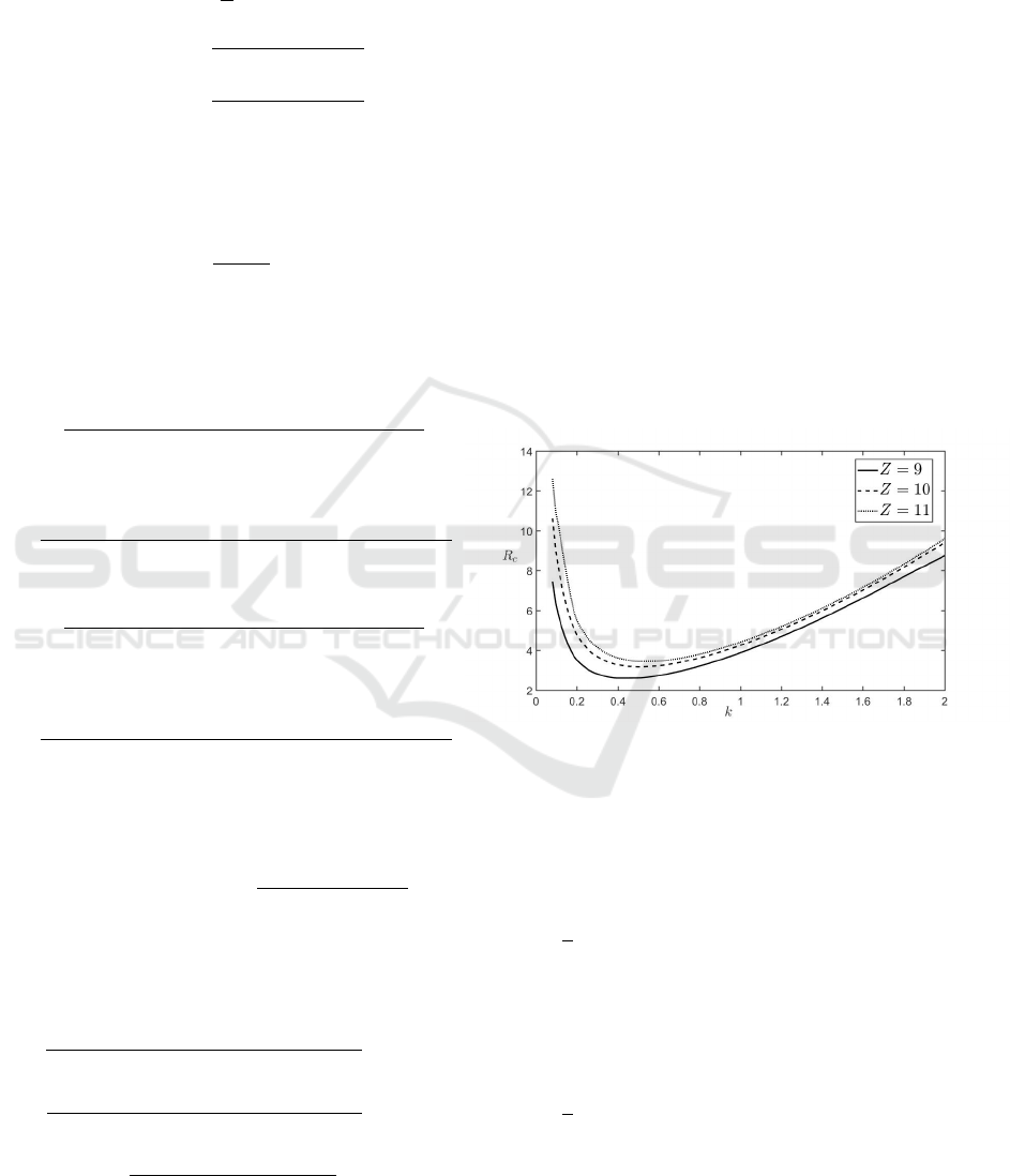
Figure 1: Critical Railey R versus wave number k for differ-
ent values of Zeldovich number Z and for V
a
= 40.
Following the same steps as in (Khalfi. O, 2016),
the interface problem is sloved by introducing the
travelling wave solution and reducing the system to
a dispersion relation. Figure 1 shows the evolution of
critical Raylaigh number R
c
as function of wave num-
ber k for different values of Zeldovich number with
u =
√
2. Here, it is remarqued that the reaction front
gains stability when Zeldovich number increases. It
can also be seen that for small values of k (k < 0.4)
the number critical Rayleig becomes very large and
R
c
increases with the wave number k when (k < 0.4).
The critical Rayleigh number R
c
versus Vadasz
number for different values of Zeldovich number with
u =
√
2 and V
a
= 40 is shown in figure 2. Here, the
lost of stablility is visible when Vadasz number V
a
in-
creases, it is also remarqued that the loss of stability
is more improtant for a bigger values of Zeldovich
number Z.
Propagation of Reaction Front in Porous Media under Natural Convection
173

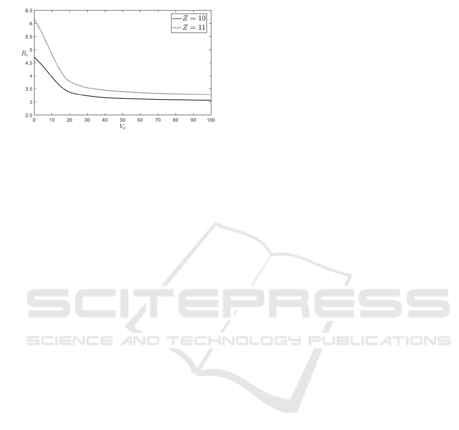
Figure 2: Critical Railey number R versus Vadasz number
V
a
for different values of Zeldovich number Z and for k =
0.5.
5 CONCLUSIONS
In this paper, we have studied a problem decribing
the reaction front propagation in porous media. The
model consists of two reaction diffusion equations of
heat and concentration coupled of those of hydrody-
namics under Darcy law.
It was observed that the key parameters of the
problem play an essential role in the convective sta-
bility of the propagating reaction front. Indeed, it was
observed that the reaction front gains stability when
Zeldovich number increases, also the lost of stablility
is remarked when Vadasz number increases.
REFERENCES
Allali, K., Ducrot, A., Taik, A., and Volpert, V. (2007).
Convective instability of reaction fronts in porous me-
dia. Mathematical Modelling of Natural Phenomena,
2(2):20–39.
Allali, Karam & Khalfi, O. (2014). On convective insta-
bility of reaction fronts in porous media using the
darcy-brinkman formulation. International Journal
of Advances in Applied Mathematics and Mechanics,
2(2):7–20.
Faradonbeh, M Rabiei & Harding, T. . A. J. . H. H. (2015).
Stability analysis of coupled heat and mass transfer
boundary layers during steam–solvent oil recovery
process. Transport in Porous Media, 108(3):595–615.
Gaikwad, SN & Kamble, S. S. (2015). Theoretical study
of cross diffusion effects on convective instability of
maxwell fluid in porous medium. American J. of Heat
and Mass Transfer, 2(2):108.
Khalfi. O, A. K. . A. C. (2016). Influence of vadasz number
on convective instability of reaction front in porous
media. American Journal of Heat and Mass Transfer,
3:37–51.
Linninger, Andreas A & Somayaji, M. R. . M. M. . Z. L.
(2008). Prediction of convection-enhanced drug de-
livery to the human brain. Journal of Theoretical Bi-
ology, 250(1):125–138.
Murphy, Ellyn M & Ginn, T. R. (2000). Modeling micro-
bial processes in porous media. Hydrogeology Jour-
nal, 8(1):142–158.
Nayfeh, A. H. (2008). Perturbation methods. John Wiley
& Sons.
Nield, Donald A & Bejan, A. (2006). Convection in porous
media, volume 3. Springer.
Stevens, Joel D & Sharp Jr, J. M. . S. C. T. . F. T. (2009).
Evidence of free convection in groundwater: Field-
based measurements beneath wind-tidal flats. Journal
of Hydrology, 375(3-4):394–409.
ICCSRE 2018 - International Conference of Computer Science and Renewable Energies
174