Solidification Behavior Study of Al-8 wt% Mg Alloy
Afaf Djaraoui
1
, Samia Nebti
2
1
Départment Sciences et Techniques, Faculté de Technologie, Université Batna2, Batna, Algérie
2
Départment de Physique, Faculté des Sciences Exactes, Université Mentouri, Constantine, Algérie
Keywords: Binary alloy, Fluent, Solidification, Simulation.
Abstract: We consider a 2D numeric simulation of the liquid-solid transition in an Al-Mg alloy. The liquid melt is
contained in an axisymmetric rectangular enclosure with isothermal walls. The heat transfer is modelled
using the Fluent V.6.3.26 code. In the unsteady state of the process, free convective fluid flows are seen
as two contra-rotating swirls. This movement is driven by the important temperature gradients generated
in the liquid region. When the steady state is established (liquid-solid equilibrium), the velocities
determining the convective flows are cancelled. The solidification proceeds then by a purely conductive
mode. The interface shape is determined during the unsteady state by the convective flows, and then,
remains unchanged until the solidification process is achieved.
1 INTRODUCTION
The numerical modelling of alloy solidification is
still a formidable task to simulate the transport of
heat and solute. Alloy's solidification is a
complicated process given that the influence of
different parameters governing the solidification
problem
(Djaraoui, 2016), (AsleZaeem, 2012),
(Djaraoui, 2009), (Zhu, 2007), (Betram-Sanchez,
2004), (McFadden, 2000), (Glicksman, 1994),
(Trivedi, 1994), (Trivedi, 1990), (Ben Amar,
1989), (Meiron, 1986). The convection
phenomenon manifesting in the melt and mushy
region is the most important factor seen its
controlling the shape, extent and advancement of
the mushy zone. The most common causes of
fluid flow in the solidification process are thermal
and solutal gradients, surface tension gradients
and external forcing agents. Natural convection
can influence the advancement of the
solidification front even in highly conductive
alloys.
The purposeof this work is to predict the
solidification evolution under thermal condition
and the role of convective transfer in a highly
conductive binary alloy. A finite volume analysis
is carried out by the Fluent V.6.3.26 code for a
two dimensional enclosure in the unsteady state
stage.
2 PROBLEM FORMULATION
2.1 Fundamentals Equations
Solidification is a process in which a solid grows
from a liquid. The treatment of this phase change
using Fluent is done considering an enthalpy-
porosity technique. The domain is divided into
three regions (liquid, solid and the mushy zone), a
liquid fraction value 

is associated with each
cell in the domain (0 for liquid, 1 for the solid and
lie between 0 and 1 for the mushy zone). The
melt – solid interface is not tracked explicitly
(Fluent® 6.2 User’s Guide), (Conde, 2004).
The equations used to solve the alloy
solidification problem are:
The energy equation:









(1)
Whereis the enthalpy, 

is the reference
enthalpy, 

is the reference temperature and


is the specific heat capacity at constant
pressure.
The liquid fraction, (

)equation:
238
Solidification Behavior Study of Al-8 wt .
DOI: 10.5220/0009771002380243
In Proceedings of the 1st International Conference of Computer Science and Renewable Energies (ICCSRE 2018), pages 238-243
ISBN: 978-989-758-431-2
Copyright
c
 2020 by SCITEPRESS – Science and Technology Publications, Lda. All rights reserved









1














0

(2)
Where

,

, are liquidus, solidus and
mushy zone temperatures respectively.
The energy conservation equation:















∆
(3)
Whereis the density,  is the fluid velocity,


is the latent heat of fusion and is the thermal
conductivity.
2.2 Boundary Condition
The simulation, which has been carried out with
the Fluent
®
v6.3.26 code, is applied to the Al-Mg
alloy. The alloy liquid is contained in a 2D
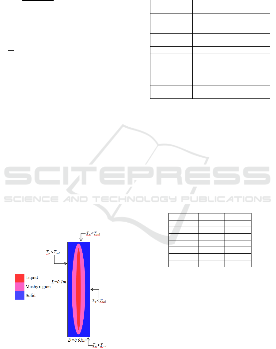
enclosure of L=0.1m height and D=0.01m width
as presented in Figure. 1. The calculation was
optimized in order to ensure an independence of
the results with respect to the grid. In order to
allow the solidification, a temperature T
w
=815K
lower than the solidus temperature of the fluid
(T
sol
), is assigned to the walls of the enclosure. In
order to study the temperature difference (T=T
0
-
T
w
) effect on the convective flow, we attributed
different values to the initial fluid temperature T
0
(820KT
0
915K). The symmetry of the problem
(horizontal and vertical) reduces the
computational domain to the 1/4 of the total
volume.The properties of the liquid melt using
aregiven in table.1.
Figure 1. Scheme of the geometrical model.
Table.1. Thermal properties of the Al-8%Mg liquid
alloy used in the calculation.
Thermal
properties
Symbol Units value
Density

Kg/m
3
2623.2
Specific heat


J/Kg.K 1085,608
Latent heat


KJ/Kg 404
Thermal
conductivity

W/m.K 221,36
Viscosity
μ
Kg/m.s 0,0013
Thermal
expansion
coefficient


K
-1
2,67. 10
-5
Solidus
temperature


K 819.82
Liquidus
temperature


K 893.15
3 RESULTS AND DISCUSSION
3.1 ∆ Effect on the Solidification
Evolution
Considering different values of T in the
solidification modelling using Fluent gives us the
results represented in table.2where t1 is the time
where the unsteady state stage is achieved and t2
represents the time of the end of the solidification
process.
Table2: Temperature difference effect on the time

T(K)
t
1
(s) t
2
(s)
5 / 0.071
10 / 0.653
20 / 1.205
30 0.244 1.531
50 0.543 1.932
70 0.761 2.201
100 0.853 2.312
It is noted that at the beginning of the
solidification process, significantT values
(T30K) create a convective movement of the
liquid melt, in the grid plane, as two contra-
rotating swirls symmetrically to the vertical axis
as it is illustrated in figure.2. The steady state is
established very quickly. For the lower T values
(T30K) we note the absence of the unsteady
state stage.
Solidification Behavior Study of Al-8 wt
239

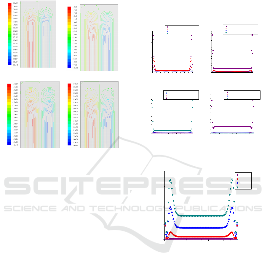
T=30K T=50K
T=70K T=100K
Figure 2. Contours of stream function (Kg/s) at t =0.1s
for different values of T.
3.2 Fluid Flow
The development of buoyancy forcesin the
enclosure plane, due to the temperature gradients,
produces a natural convection movement. The
presented flow fields are at time t=0.1s. As
exposed in figure.2, the hot fluid is guided
upwards and once reaching the cold wall, the
flow is separated into two parts deviated on the
right and on the left in a movement downwards
symmetrically to the vertical axis. The two flow
parts meet at the bottom of the enclosure in an
ascending movement giving two swirls contra-
rotating, in the enclosureplan, separated by the
symmetry axis. In the T=70K case, each of the
two vorticesis divided into three parts: two small
vortices (close to horizontal walls) and a main
vortex between them. Within the small vortices,
flow particles cannot follow the accelerated
motion of the main vortex along the vertical wall
and they are deviated towards the middle of the
enclosure. This deviation may be explained by
the weak momentum of the fluid particles within
the small vortices. However, for T=100K, at the
specified time, the flow field is represented by the
two swirls contra-rotating, in the plan of the
enclosure, and we notice the absence of the small
swirls. At this time, the mentioned small vortices
have already merged with the main swirls
because of the faded motion of the main swirls.
0,00 0,02 0,04 0,06 0,08 0,10
0,000000
0,000005
0,000010
0,000015
0,000020
0,000025
t=0.1s
t=0.244s-end of unsteady state stage-
t=1s
t=1.531s-end of solidification-
Velocity magnitude
(M/s)
Y Posi tion
(m)
0,00 0,02 0,04 0,06 0,08 0, 10
0,00000
0,00002
0,00004
0,00006
0,00008
0,00010
0,00012
0,00014
0,00016
0,00018
t=0.1s
t=0.543s-end of unsteady state stage-
t=1s
t=1.932s-end of solidification-
Velocity magnitude
(m/s)
Y Position
(m)
T=30K T=50K
0,00 0,02 0,04 0,06 0,08 0,10
0,0000
0,0002
0,0004
0,0006
0,0008
t=0.1s
t=0.761s-end of unsteady state stage-
t=1s
t=2.201s-end of solidification-
Velocity magnitude
(m/s)
Y Pos ition
(m)
0,00 0,02 0,04 0,06 0,08 0,10
0,0000
0,0002
0,0004
0,0006
0,0008
0,0010
t=0.1s
t=0.853s-end of unsteady state stage-
t=1s
t=2.312s-end of solidification-
Velocity magnitude
(m/s)
Y Position
(m)
T=70K T=100K
Figure 3. Velocity magnitude curves for different T
values.
0,00 0,02 0,04 0,06 0,08 0, 10
0,000000
0,000001
0,000002
0,000003
0,000004
T=30K
T=50K
T=70K
T=100K
Velocity magnitude
(m/s)
Y Position
(m)
Figure 4. Velocity magnitude curves for different T
values at the vertical axis (x=0.005m) at t=1s.
Figures 3 and 4 indicate that the important
temperature difference(T=100K) has the
maximal magnitude velocity and so generates an
important convective movement of the liquid
melt.
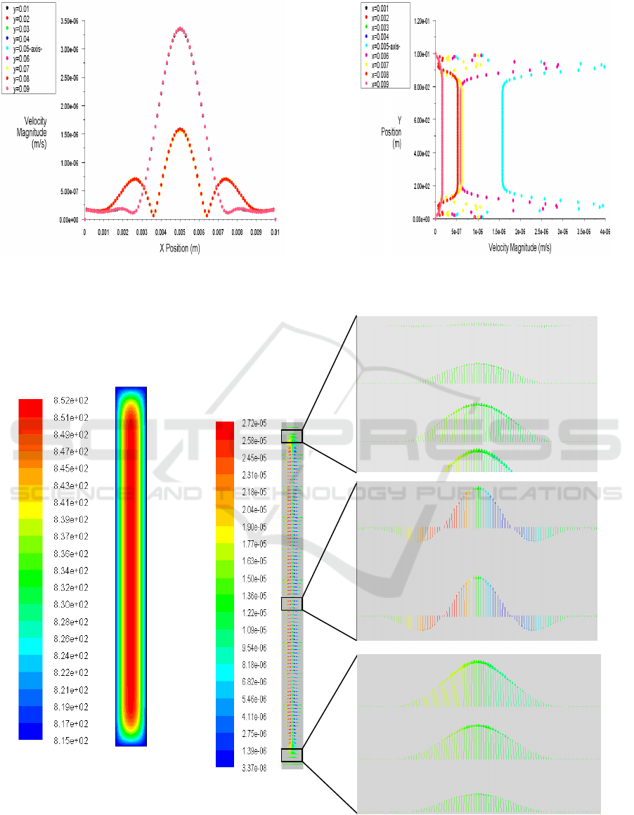
As it is shown in figure.5, the velocity is
maximal (v= 3.510
-6
m/s)for y=0.01m and
y=0.09m (near the walls) and constant for each
other y. The velocity is maximal for x=0.05m and
it decreases for each other x points, which
indicates that important convective current results
in the enclosure centre.
240

(a) (b)
Figure 5. Velocity magnitude for T=100K at t=1s.
Contours of static
temperature
Velocity vectors colored by stream function (Kg/s)
Figure 6. Temperature difference effect on the convective movement at t =0.8s (before the end of the unsteady state
stage) for T=100K.
Solidification Behavior Study of Al-8 wt
241

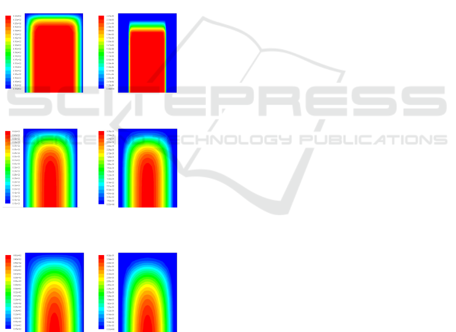
Figure.6illustrates that the liquid flowdepends
on the temperature gradient: Near the up and the
down walls the convective movement flow one
direction. In the geometry centre, the liquid flow
is governed by the density variations which is
strongly influenced by the temperature gradients
3.3 Temperature Field
The temperature differencesimplicate the
generation of the driving thermal force, which
provokes a natural convectionmovement. The hot
liquid is driven upwards and once reaching the
cold wall, it is separated into two parts by the
vertical symmetry axis. In the bottom, the two
parts meet in an upswing thus creating two
vortices contra-rotating divided by the vertical
symmetry axis. This phenomenon is illustrated in
figure.7 (contours of static temperature).
Contours of static Contours of liquid
temperature at t=0.01s fraction at t=0.01s
T=5K
Contours of static Contours of liquid fraction
temperature at t=0.244s at t=0.244s(end of the non
(end of the non steady state)steady state)
T=30K
Contours of static Contours of liquid fraction
temperature at t=0.853s at t=0. 853s(end of the(end of
the non steady state) non steady state)
T=100K
Figure 7. Contours of static temperature and liquid
fraction.
3.4 Liquid Fraction
Looking at the contours of liquid fraction
representing in Figure. 7, we can assume that the
same behaviour, detecting for the temperature
contours, is observed for the contours of liquid
fraction
4 CONCLUSION
During the solidification process, the motion of
the Al-Mg liquid melt is initially driven by the
temperature gradients. An unsteady state stage
appears for important values of temperature
differences between the walls and the liquid alloy
temperatures (T30K). Free convective fluid
flows are generated as two contra-rotating swirls.
For T=70K, the two contrarotative swirls are
divided into three parts. Two satellites are
created, limiting a central swirl, in the upwards
and the downwards of the enclosure. When the
steady state is established (liquid-
solidequilibrium), the velocities determining the
convective flows are cancelled. The solidification
proceeds then by a purely conductive mode. The
interface shape is determined during the unsteady
state stage by the convective flows, and then,
remains unchanged until the solidification
process is achieved.
REFERENCES
Djaraoui, A., & Nebti, S. (2016). On the Origin of Grid
Anisotropy in the Simulation of Dendrite Growth
by a VFT Model. Metallurgical and Materials
Transactions A, 47(10), 5181-5194.
Zaeem, M. A., Yin, H., & Felicelli, S. D. (2012).
Comparison of cellular automaton and phase field
models to simulate dendrite growth in hexagonal
crystals. Journal of Materials Science &
Technology, 28(2), 137-146.
Djaraoui, A., Nebti, S., Noui, S., (2009). Analysis of
no-steady state stage during rapid solidification of
an Al-Mg alloy, 9ème Congrès de Mécanique, FS
Semlalia, Marrakech.
Zhu, M. F., & Stefanescu, D. M. (2007). Virtual front
tracking model for the quantitative modeling of
dendritic growth in solidification of alloys. Acta
Materialia, 55(5), 1741-1755.
Zhu,M. F., Stefanescu, D. M., 2007. Virtual front
tracking model for the quantitative modeling of
dendritic growth in solidification of alloys, Acta
Materialia, 55: 1741-1755,.
242

Beltran-Sanchez, L., &Stefanescu, D. M. (2004). A
quantitative dendrite growth model and analysis of
stability concepts. Metallurgical and Materials
Transactions A, 35(8), 2471-2485.
Conde, R., Parra, M. T., Castro, F., Villafruela, J. M.,
Rodrı
́
guez, M. A., & Méndez, C. (2004).
Numerical model for two-phase solidification
problem in a pipe. Applied thermal engineering,
24(17-18), 2501-2509.
McFadden, G. B., Coriell, S. R., & Sekerka, R. F.
(2000). Effect of surface free energy anisotropy on
dendrite tip shape. Acta materialia, 48(12), 3177-
3181.
Glicksman, M. E., Koss, M. B., & Winsa, E. A. (1994).
Dendritic growth velocities in microgravity.
Physical review letters, 73(4), 573.
Trividi, R. K., Kurz, W. (1994). Dendritic growth.
International Materials Review, 39: 49-74.
Trivedi, R. K., Mason, J. T.(1990). The effect of
interface kinetics on solidification interface
morphologies. Metallurgical Transactions A,21,
235-249.
Ben Amar, M., Pelce, P. (1989). Impurity effect on
dendritic growth . Phys rev A, 39, 4263.
Meiron,D. I.(1986).Selection of steady states in the
two-dimensional symmetric model of dendritic
growth.Phys Rev A, 33, 2704.
Fluent® 6.2 User’s Guide.
Solidification Behavior Study of Al-8 wt
243