The Analysis of Interdependency Macroeconomic Variables of

Rupiah Exchange Rate Volatility using Vector Auto Regression

Period 2008-2017

Masnia Nasution

, Dede Ruslan

and Andri Zainal

Post Graduate of Economics, State University of Medan, Medan-Indonesia

Faculty of Economics, State University of Medan, Medan-Indonesia

Keywords: Rupiah Exchange Rate Volatility, Macroeconomic Variables, VAR

Abstract:

Understanding volatility of rupiah exchange rate very important because interdependency of macro

economic variables. Fluctuation one of macroeconomic variables then rupiah exchange rate volatility certain

follow moving appreciation or depreciation suspend from fast or slow fluctuation one of macroeconomic

variables. Dornbusch theory state with the concept of "Overshooting" (soaring/fluctuating) with the

"Monetary Sticky Price" model. The basis of this model is the uncertainty of fluctuating high rupiah

exchange rate volatility. This study explores how the interdependence of macroeconomic variables on

rupiah exchange rate volatility. The data used series time data were conducted that accepted from Economic

and Financial Statistics Bank of Indonesia during the period of 2008-2017. The methods used in this

research were Vector Autoregression (VAR). The results of the study concluded that (1) in the short term

dominant cointegration towards inflation, the money supply, the export of non-oil and gas commodities (2)

while the medium term cointegration towards interest rates (3) and while in the long term cointegration of

gross domestic product (4) In addition, non commodity export shocks Oil and gas in the short term does not

provide a dominant contribution to the volatility of the rupiah exchange rate, in the medium term interest

rates make a dominant contribution to the volatility of the rupiah exchange rate, and in long-term growth

(GROW) make a dominant contribution to the volatility of the rupiah. Government policy simulations

emphasize interest rates to 6.5 percent so that inflation can subside after the 2008 global crisis, but not

reduce the money supply and increase economic growth, the government is important to simulate other

policies to better anticipate the global crisis.

1 INTRODUCTION

Economic and financial stability is currently

inseparable from changes in the development of

macroeconomic variables that affect the volatility of

the rupiah exchange rate. One of the changes in the

development of macroeconomic variables is that

they are unstable, which can result in a turbulent

global financial crisis that has changed the world

economic order, especially Indonesia, and has a

significant effect on the volatility of the rupiah

(Bank Indonesia, 2016).

One of the theories of exchange rate volatility is

that introduced by Rudi Dornbusch (in Pilbeam,

2016) using the concept of "Overshooting" with the

"Sticky hgjsMonetary Price" model. The basis of

this model is the uncertainty of soaring high

exchange rate volatility. With the concept of

overshooting the exchange rate, it is assumed that

there are several parts of the economy that cause

instability from other parties, especially the

exogenous variables change, which results in short-

term effects on exchange rates that can be greater or

higher in long-term effects so that the exchange rate

exceeds its value in the long run. One exogenous

variable changes as the high interest rates affect the

depreciation of the exchange rate in the short term so

that the possibility of price increases can be

followed by exchange rate behavior, the

overshooting trend of exchange rates is in the long

run.

As is known by the phenomenon that has

occurred in Indonesia in 1997/1998, there was an

economic crisis in which the turbulent

macroeconomy which quickly affected economic

fundamentals through the exchange rate channel.

634

Nasution, M., Ruslan, D. and Zainal, A.

The Analysis of Interdependency Macroeconomic Variables of Rupiah Exchange Rate Volatility using Vector Auto Regression Period 2008-2017.

DOI: 10.5220/0009510306340642

In Proceedings of the 1st Unimed International Conference on Economics Education and Social Science (UNICEES 2018), pages 634-642

ISBN: 978-989-758-432-9

2000

4000

6000

8000

10000

12000

14000

16000

I III I III I III I III I III I III I III I III I III I III

2008200920102011201220132014201520162017

ExchangeRate

0.00%

2.00%

4.00%

6.00%

8.00%

10.00%

12.00%

14.00%

I IIIIIIVI IIIIIIV I IIIIIIVI IIIIIIV I IIIIIIVI IIIIIIV I IIIIIIVI IIIIIIV I IIIIIIV I IIIIIIV

2008 2009 2010 2011 2012 2013 2014 2015 2016 2017

1000000

2000000

3000000

4000000

5000000

6000000

IIIIIIIVI IIIIIIVI IIIIIIVI IIIIIIVI IIIIIIVI IIIIIIVI IIIIIIVI IIIIIIVI IIIIIIVI IIIIIIV

2008200920102011201220132014201520162017

Assuming, from Dornbush's theory that there are

several macroeconomic variables such as inflation,

interest rates, and the money supply that affect

exchange rate volatility, where price increases will

create supply of goods which will increase relative

prices of domestic goods as a result of exchange

rates depreciated by 8,025 Rupiah/USD (Indonesian

Economic Report, 1998) so interest rates were also

high through behavioral balance in the money

market so that the money supply increased which

caused slow and depressed exchange rate

movements in the short term.

From this study it can be concluded that

exchange rate volatility applies to free floating

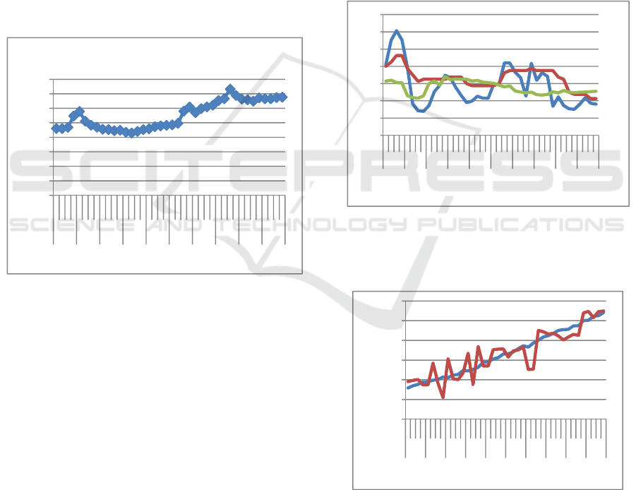
systems. From this phenomenon can be presented a

graph of the development of rupiah exchange rate

volatility from 2008 to 2017 in Figure 1. is Volatility

of Exchange Rate

Figure 1: Volatility of Exchange Rate

Source: Bank of Indonesia

From the graph it can be seen that the rupiah

exchange rate over the past ten years has fluctuated

quite as much as in 2008, 2013 and 2015. However,

consistent and prudent macroeconomic policies

accompanied by exchange rate stabilization

measures can generally reduce the pressure

excessive. Despite being hit by a variety of

fluctuations, the rupiah exchange rate moved

steadily from 2009 to 2013 in quarter III. However,

the impact of the wider global financial crisis

triggered a significant amount of asset release by

investors, which caused strong pressure on the

rupiah exchange rate during the third quarter of

2015. In 2015 in the quarter III the rupiah exchange

rate volatility experienced depreciation at the level

of Rp. 14,657, but in the fourth quarter of 2015 the

exchange rate volatility appreciated until the fourth

quarter of 2016 which had a good impact on

macroeconomic variables with 5.5 percent inflation

in 2016 to 4.25 percent. In 2017, the decline caused

by macroeconomic variables, the BI rate interest rate

rose above inflation, triggering the growth of the real

sector and declining capital costs and increasing

demand for banks which could then increase

economic growth.

Judging from the trend above, which causes the

development of exchange rate volatility inevitably

fluctuates from the impact of macroeconomic

variables. Next in Figure 1.2. is inflation, interest

rates, and gross domestic product

presented graphs of developments in inflation,

GDP, interest rates, JUB, and commodity exports

(non-oil and gas) that affect the volatility of the

rupiah exchange rate in 2008-2017.

Figure 2: Inflation, interest rates, and gross domestic

product

Figure 3: Money supply and commodity exports of

non-oil and gas

Source: SEKI, Bank of Indonesia

When seen the volatility trend of the rupiah

exchange rate in the past decade has depreciated, it

shows that the rupiah has declined against the US

dollar due to the global crisis. Figure 1.2 (a),

The Analysis of Interdependency Macroeconomic Variables of Rupiah Exchange Rate Volatility using Vector Auto Regression Period

2008-2017

635

inflation shows a rising trend due to world oil prices

reaching 9.2 percent so the inflation trend reaches

11.06 percent and experienced a significant

economic slowdown of 6.01 percent. At the same

time, BI emphasized the interest rate (BI Rate) was

much lower, emphasizing interest rates would have

an impact on increasing the money supply (Pohan,

2008). But from the post-global crisis BI focused its

financial performance so that the economic crisis

could subside which was done by emphasizing the

price of oil to be cheaper and sharp enough to lower

oil prices so that inflation could subside around 2.78

percent so that the inflation trend declined and

returned within the target range the country

especially Indonesia to emphasize lower interest

rates and improve economic growth towards a

positive direction.

The decline in domestic inflation, in theory is

very much responded by the public to reduce the

price of commodity goods, the world of work to

increase employment and reduce unemployment,

and rising economic growth towards a positive

direction for the welfare of society. Likewise, the

trend in the interest rate in 2010 began to decline

due to appreciation in the rupiah exchange rate

appreciation, but JUB continued to show

improvement. The rupiah exchange rate during the

2011-2012 period has weakened to depreciate

against the US dollar, as shown in Figure 1.2 (a) is

inflation, interest rates, and gross domestic product)

where the same year inflation, interest rates indicate

a decline and economic growth also slowed by 6.11

percent, seen from Figure 1.2 (a) is inflation, interest

rates, and gross domestic product) so trend inflation,

interest rates, and economic growth intersect with

JUB in fact increase as in Figure 1.2 (b) is money

supply and commodity exports of non-oil and gas).

Seeing the condition of the rupiah exchange rate

increase, exports of goods will also increase abroad.

The export price of the goods tends to be cheap

compared to the prices of domestic goods, which

causes the supply of goods both domestic and

foreign to increase, in turn, will reduce the price of

the goods so that the CPI must be able to be

controlled with the target can help the inflation

process towards lower long term. And it is seen that

the inflation trend in 2012 has slightly increased, this

indicates that a significant increase in JUB can cause

the inflation rate to rise.

2 THEORICAL FRAMEWORK

2.1. Rupiah Exchange Rate Volatility

Overshooting exchange rates can occur when

exchange rates adjust faster than goods and services.

Dornbusch treats the exchange rate as a jump

variable where the exchange rate adjusts quickly to

the disruption of the economy, while other variables

such as output, price, and interest rates are in

adjustment to be slow to barely move. Dornbusch

extends the version of the perfect capital mobility

from Mundel-Fleming. Dornbusch includes

exchange rate expectations to explain volatility in

exchange rates and include dynamic elements

(Dornbusch, 1980).

The characteristics of the Dornbusch model are

sticky prices in the short term. Overshooting the

model involves the process of adjusting in exchange

rates and immovable prices at the same speed level.

Suppose there is a monetary expansion. Short-term

expansion of monetary policy causes interest rates to

fall. This reduction in interest rates immediately

pushes adjustments in exchange rates but prices

adjust gradually. In response to a shock to the

economy, the exchange rate will be overshooting the

level of balance. First of all the exchange rate will

move to a level above the balance then it will

gradually return to the long-term balance.

2.2. Macroeconomic Variables

Macroeconomics is a branch of economics that

studies the phenomenon of economic indicators in

aggregate or whole, for example economic growth,

unemployment, inflation, interest rates, circulation

of money in an economy. Macroeconomic

explanations include economic changes that affect

all households, companies, and markets simultan

(Mankiw, 2004: 500). And there are also four keys

in the macro market, namely (1) natural resources,

(2) exports of goods and services or commodities,

(3) loanable funds, and (4) foreign exchange

(exchange rates) (Sobel, 2009).

Inflation

Inflation is one indicator of macroeconomic

variables in analyzing the economy of a country,

especially related to the broad impact on aggregate

macroeconomic variables. According to Lerner

(Gunawan, 1995), inflation is a situation where there

is an excess demand for goods and services as a

whole. According to Keynesian theory, inflation is

an excess of money supply compared to demand and

without expansion of money supply, excess

aggregate demand can occur if the increase in

consumption expenditure, investment, government

expenditure, and exports, thus inflation can be

caused by monetary and non-monetary factors

(Gunawan, 1995).

UNICEES 2018 - Unimed International Conference on Economics Education and Social Science

636

Interest rate

Interest rate stability is expected, because the

stability of interest rates also encourages financial

market stability so that the ability of financial

markets to channel funds from people who have

productive investment opportunities can run

smoothly and economic activities also remain stable

According to Mishkin (2008: 60) and interest rates

are one indicator of macroeconomic variables in

analyzing the economy of a country is mainly

related to the widespread impact on macroeconomic

variables in the aggregate (Gunawan, 1995).

Therefore, Bank Indonesia is in charge of

maintaining the stability of interest rates to create a

more stable financial market.

Gross Domestik Product

According to Robert B. Barsky in N. Gregory

Mankiw (2005; 15), Gross Domestic Product (GDP)

is the total income from the production of goods

equal to the amount of wages and profits in the

upper half of the circulation of money. Gross

Domestic Product (GDP) is the market value of coal

and final services produced in the economy for a

certain period of time. GDP is often considered the

best measure of economic performance. This

statistic is calculated every three months by the

Bureau of Economic Analysis from a large number

of primary data sources. The goal of GDP is to

summarize economic activity in the value of a single

currency over a long-term period.

Money Supply

The amount of money is one of the indicators of

economic macro variables, which in the form of

capital, which are based on the balance of the

quantity of money. The amount of money is in the

wild (just supply) holding the investor in the

economy of a country. The amount of money that is

released in the economy of a country will be able to

give a boost to the exchange rate of its currency

against foreign currencies. The increase in the offer

of money or the amount of money will increase the

price of goods which are measured by the value of

money and will also increase the price of foreign

exchange measured by the domestic currency

(Triyono, 2008).

Exports Of Non-Oil And Gas Commodities

Countries that have implemented an open economic

system will interact freely with other economies

throughout the world. One of the activities of

international economic interaction is by conducting

commodity exports (Non-oil and gas). According to

Tietenberg (2014: 149) that commodity exports

(non-oil and gas) are energy resources that are

endless and renewable. Resources (Non-oil and gas)

do not have a limited amount at a certain time so that

if the resources are depleted, this will certainly not

interfere and will not hinder the sustainability of

economic development. The non-oil and gas sector

consists of the agriculture, mining and minerals sub-

sectors, as well as the processing industry. These

three non-oil and gas subsectors have important

contributions to Indonesia's economic and financial

growth.

3 RESEARCH METHOD

This study discusses the analysis of interdependency

of macroeconomic variables on the volatility of the

rupiah exchange rate. This study use the Vector

Auto Regression (VAR) method to see the short and

long term endogenous variables which are

considered to have interdependence between

macroeconomic variables towards the volatility of

the rupiah exchange rate. The type of data used in

this study is secondary data that is time series in the

observation period Q: 1 2008 up to Q: IV 2017. The

data sources used for this study are allowed from

Indonesia Financial and Economic Statistics (SEKI)

published by Bank of Indonesia (BI), the Indonesian

Economic Report (LPI), and the Central Statistics

Agency (BPS).

The Vector Auto Regression (VAR) method first

proposed by Sims (1980) appears as a solution to the

problem of the complexity of estimation and

inference processes because of the presence of

endogenous variables on both sides of the equation

(variable endogeneity) which are dependent and

independent. While economic theory alone as a basis

for consideration of simultaneous equations will not

be sufficiently complete in providing strict and

precise specifications for dynamic relationships

between variables (Yahya, 2017).

The VAR stage is to do stationary testing of the

data used in determining the maximum lag and

optimal lag that will be used to perform stationary

tests, cointegration tests, estimation of the VAR

model, impulse response, and variance

decomposition.

The Analysis of Interdependency Macroeconomic Variables of Rupiah Exchange Rate Volatility using Vector Auto Regression Period

2008-2017

637

Stationary Data Test (Root Test Unit / Unit Root

Test)

The first step in processing time series data is by

testing stationarity or unit root test. Stationary data

will tend to approach average values and fluctuate

around the average or have a constant range. If the

data is stationary, then the method chosen is the

VAR method and if it is not stationary then use the

VECM method. (Ayyuniyyah, Laily and Beik,

2013). The assessment of Dickey and Fuller's

methods (Gujarati, 1998) are as follows:

∆







 







∆







where:

Y = observed variable

Δ =  −  – 1

T = time trend

Cointegration Test (Optimal Lag Length)

To determine the length of lag used supporting

parameters, namely: AIC (Akaike Information

Criterion), SIC (Schwarz Information Criterion), and

LR (Likelihood Ratio). Determination of the number

of lags used from the VAR equation with AIC, SIC,

or LR is the smallest amount of lag. The value of

AIC, SIC, or LR is useful for choosing the best

model. However, if there is a contradiction between

the values of AIC, SIC, and LR, the criteria of SIC is

used because the SIC criteria provide a scale that is

greater than the other criteria.

According to Enders (2014) the calculations of

AIC and SC are as follows:

AIC (k)= ln







where:

T = number of observations used

K = lag length

SSR = Redisual Sum of Squares

N = number of money parameters estimated

Johansen Cointegration Test

In this study the cointegration test used was the

cointegration test developed by Johansen. This test

can be used to determine the cointegration of a

number of variables (vectors). In the Johansen

cointegration test carried out with two statistical

tests, the first to test the null hypothesis can use trace

test statistics which require that the number of

cointegration directions is less than or equal to p and

this test can be done as follows:

trace(r) = -T i

∑





(1-i)

where:

 + 1, ...  declares the value of the smallest

eigenvectors ( − ).

Vector Auto Regression (VAR) of Analysis Model

VAR is a system and equation with the number of

endogenous variables as much as n. VAR is a

multivariate time series which assumes that all

variables are endogenous variables. Sims (1980)

states that there is true simultaneity between all

variables. Then all related variables must be treated

correctly, there must be no difference in treatment

between endogenous and exogenous variables.

Enders (2014) formulates primitive first order

bivariate systems which are written as follows:

yt = b10–b12 zt+γ11 yt-1+γ12 zt-1+εyt

Impulse Response Function (IRF)

Impulse Response is one of the important analyzes

in the VAR / VECM model. This impulse response

analysis tracks the response of endogenous variables

in the VAR / VECM system due to shock or changes

in the disturbance variable (e). The impulse response

in this study was conducted to determine the

interdependence response of macroeconomic

variables to the volatility of the rupiah exchange

rate.

Forecasting Error Variance Decomposition

In addition to the impulse response in the VAR /

VECM model it also provides analysis of

Forecasting Error Variance Decomposition or often

called variance decomposition. In a variance

decomposition, it can be seen the relative

importance of each variable in the VAR / VECM

system due to shock. Variance decomposition is

useful for predicting the contribution percentage of

each variable due to changes in certain variables in

the VAR / VECM system.

Granger Causality Analysis

In economic analysis, the causal relationship

between variables does not only run in one direction.

So through the granger causality test in essence it

can indicate whether a variable has a two-way

relationship or only one direction. In regression

analysis, even though we have made the influence of

one variable on other variables, it is not explained

the direction of the relationship of the variable. In

other words, the extension of the relationship

between variables does not indicate causality or

direction of the relationship. Causality Test

generally uses a test developed by Genger, with the

Granger Causality Test method.

Equation models that can be formed from the

above conditions are:

 ∝



∝



∝



∝





∝



∝





UNICEES 2018 - Unimed International Conference on Economics Education and Social Science

638

where:

Y : Dependent Variable (NTR)

∝_0 : constants

∝_1 : matrix parameter n x n, for every 1 = 1, 2, ... p

X_1 : INF

X_2 : SB

X_3 : GDP

X_4 : JUB

X_5 : EXKNM

To reinforce the causality model above, an F-

Test can be done for each regression. To test the

hypothesis, the F test is used as follows:













/











where :

m = number of lags

k = number of parameters estimated in unrestricted

regression

4 ANALYSIS

This research is a follow-up study from previous

studies that produced a design method of analysis

that produces about:

Development of Volatility in Rupiah Exchange

Rates

Throughout 2008 to 2017, there were three peaks

where the exchange rate volatility depreciated,

namely in 2008, 2013, and 2015 where in all three

years all goods needs rose continuously which

resulted in a weak rupiah exchange rate. However,

consistent and prudent macroeconomic policies

accompanied by measures of exchange rate

stabilization can generally reduce the occurrence of

excessive pressure. Despite being hit by a variety of

fluctuations, the rupiah exchange rate moved

steadily from 2009 to 2013 in quarter III. However,

the impact of the wider global financial crisis

triggered a significant amount of asset release by

investors, which caused strong pressure on the

rupiah exchange rate during the third quarter of

2015.

In general, the volatility of the rupiah exchange

rate experienced instability until the end of

December 2015. It began the volatility of the

exchange rate in 2008 in Q4 IV at the level of Rp.

10,950 per US dollar due to the inflation rate of

11.06 percent resulting in an increase in world prices

and a drop in commodity prices which depressed the

rupiah, so that the rupiah exchange rate depressed.

In 2013, in Q4 IV there was volatility in the rupiah

exchange rate experiencing instability at the level of

Rp. 12,250 due to the interest rate (BI) rate

increasing until early 2014 from 5.75 percent to 7.75

percent in the fight against the depreciating rupiah

which limited the foreign exchange liquidity and

balance of payments deficit.

In 2015 in the quarter III the rupiah exchange

rate volatility experienced depreciation at the level

of Rp. 14,657, but in the fourth quarter of 2015 the

exchange rate volatility appreciated until the fourth

quarter of 2016 which had a good impact on

macroeconomic variables with 5.5 percent inflation

in 2016 to 4.25 percent. In 2017, the decline caused

by macroeconomic variables, thes BI rate interest

rate rose above inflation, triggering the growth of the

real sector and declining capital costs and increasing

demand for banks which could then increase

economic growth.

Development of Macroeconomic Variables

Macroeconomic variables used in this study are

inflation, interest rates, gross domestic product,

money supply, and exports of non-oil and gas

commodities. This macroeconomic variable is also

an endogenous variable which is considered to have

an interdependence between the variable volatility of

the rupiah exchange rate.

The following is briefly explained the

development of macroeconomic variables used in

this study, as follows:

In the fourth quarter of 2008 there was a global

crisis where all goods needs increased due to world

oil prices reaching 9.2 percent so the inflation trend

reached 11.06 percent and experienced a significant

economic slowdown of 6.01 percent. At the same

time, BI emphasized the interest rate (BI Rate) was

much lower, emphasizing interest rates would have

an impact on increasing the money supply (Pohan,

2008). But from the post-global crisis BI focused its

financial performance so that the economic crisis

could subside which was done by emphasizing the

price of oil to be cheaper and sharp enough to lower

oil prices so that inflation could subside around 2.78

percent so that the inflation trend declined and

returned within the target range the country

especially Indonesia to emphasize lower interest

rates and improve economic growth towards a

positive direction.

The decline in domestic inflation, in theory is

very much responded by the public to reduce the

price of commodity goods, the world of work to

increase employment and reduce unemployment,

and rising economic growth towards a positive

The Analysis of Interdependency Macroeconomic Variables of Rupiah Exchange Rate Volatility using Vector Auto Regression Period

2008-2017

639

direction for public welfare. Likewise, the trend in

the interest rate in 2010 began to decline due to

appreciation in the rupiah exchange rate

appreciation, but JUB continued to show

improvement. The rupiah exchange rate during the

2011-2012 period has weakened to depreciate

against the US dollar, where with the same year

inflation, interest rates indicate a decline and

economic growth also slowed by 6.11 percent but

the amount of money in circulation is still increasing

where Indonesian banks cannot attract the amount of

money in society to be reduced so that economic

growth does not continue to slow down and even the

volatility of the rupiah exchange rate continues to

depreciate to date.

5 RESULTS

Stationarity Test

The augmented Dickey Fuller Test (ADF test)

results on the NTR (Rupiah Exchange Rate), INF

(Inflation), Interest Rate, GDP (Gross Domestic

Product), JUB (Money Supply), the EKNM (Export

of Non-oil Commodities) are presented in table 1

below:

ull Hypothesis: Unit root (individual unit

root process)

Series: Y, X1, X2, X3,

X4, X5

Date: 08/17/18

Time: 12:44

Sample: 2008 2017

Exogenous variables: Individual effects

Automatic selection of maximum lags

Automatic lag length selection based on SIC: 0 to

Total number of observations: 224

Cross-sections included: 6

Tabel 1:Unit Root Test

Method Statistic Prob.**

ADF-Fisher Chi square 142.733 0.0000

ADF - Choi Z-stat 10.3213 0.0000

** Probabilities for Fisher tests are computed

using an asymptotic Chi-square distribution. All

other tests assume asymptotic normality.

Intermediate

ADF test results D (UNTITLED)

Series Prob. Lag MaxLag Obs

D(Y) 0.0001 0 9 38

D(X1) 0.0000 0 9 38

D(X2) 0.0014 0 9 38

D(X3) 0.0013 3 9 35

D(X4) 0.0000 0 9 38

D(X5) 0.0000 1 9 37

All variables of the Prob value. His <0.05, it is

stationary at first difference. At first different the

stationary has been tested then the results are

stationary so we continue with the regress VAR

Cointegration Test

Cointegration tests are conducted to see whether

among the variables there are cointegrated, either

randomly or irregularly, at least among the variables

there is one that is cointegrated. Based on the results

of the tests carried out, the results obtained as shown

in table 5.2 are;

VAR Lag Order Selection Criteria

Endogenous variables: D(Y) D(X1) D(X2) D(X3) D

(X4) D(X5)

Exogenous variables: C

Date: 08/17/18 Time: 20:16

Sample: 1 40

Included observations: 36

Table 2: Lag Optimal Test

Lag LogL LR FPE AIC

0 -1367.740 NA 5.62e+25

76.31887

1 -1328.157 63.77176

4.75e+25 76.11985

2 -1296.410 40.56647

7.16e+25 76.35609

3 -1236.229 56.83708*

3.10e+25* 75.01273*

* indicates lag order selected by the criterion

LR: sequential modified LR test statistic

(each test at 5% level)

FPE: Final prediction error

IC: Akaike information criterion

SC:Schwarz information criterion

HQ: Hannan-Quinn information criterion

From the results obtained, it is known that the

optimum lag is 3 which is indicated by the most

number of asterisks (*) in lag 3

Vector Auto Regression (VAR) of Analysis Model

VAR Model - Substituted Coefficients:

===============================

D(Y)=-0.113884585481*D(Y(-1))- 0.715797471729*

D(Y(-2))-0.481357171336*D(Y(-3))+ 33.4506413885

*D(X1(-1))+18.9930119224*D(X1(-2))+ 172.743648

182*D(X1(-3))+362.822243193*D(X2(-1))+ 25.7217

477862*D(X2(-2))+233.526150069*D(X2(-3))-392.8

UNICEES 2018 - Unimed International Conference on Economics Education and Social Science

640

00381611*D(X3(-1))-508.691804752*D(X3(-2))-153.

144651134*D(X3(-3))- 0.000871801654563*D(X4(-

1))+0.00269698056232*D(X4(-2))+0.00369735260

857*D(X4(-3))+0.000143214123963*D(X5(-1))+ 0.00

0139759923035*D(X5(-2))+1.88664763183e-05*D

(X5(-3)) - 267.534125709

D(X1)=-0.00173481077078*D(Y(-1))-0.0007770487

53329*D(Y(-2))-0.000662930817514*D(Y(-3))-0.165

411884068*D(X1(-1))+0.178791377505*D(X1(-2))+

0.121916249943*D(X1(-3))+1.21958232882*D(X2(-

1))-0.00721322599839*D(X2(-2))- 0.61870857 3721*

D(X2(-3))-0.560009053009*D(X3(-1))+0.297779289

534*D(X3(-2))+0.235196122872*D(X3(-3))+7.29514

99098e-06*D(X4(-1))+8.64014501021e-06*D(X4(-2))

+ 1.5361745813e-06*D(X4(-3)) + 2.01008955641e-

07*D(X5(-1))-1.65476499611e-07*D(X5(-2))- 2.8712

9019645e-07*D(X5(-3))-1.39391241196

D(X2)=-0.000294444597221*D(Y(-1))-0.000119120

145977*D(Y(-2))+0.000107270155489*D(Y(-3))+0.1

33710901718*D(X1(-1))+0.125197005184*D(X1(-2))

+0.0217702739235*D(X1(-3))+0.255648641462*D

(X2(-1))+0.00532231118813*D(X2(-2))-0.37995815

0987*D(X2(-3))-0.521702148326*D(X3(-1))-0.0216

829604442*D(X3(-2))-0.156936321447*D(X3(-3))+

7.28529712477e-07*D(X4(-1))+1.0713054295e-06*

D(X4(-2))+4.97909411856e-07*D(X4(-3))-1.165150

23832e-07*D(X5(-1)) - 2.56920654825e-07*D(X5(-

2))-2.84626707384e-07*D(X5(-3))-0.227443958008

D(X3)=-0.000229917029967*D(Y(-1))+7.174258162

81e-05*D(Y(-2))+5.16065758101e-05*D(Y(-3))+0.03

21609063049*D(X1(-1))-0.0789446848571*D(X1(-2)

)-0.0999994252515*D(X1(-3))+0.300218933817*D

(X2(-1))-0.0709165261706*D(X2(-2))-0.332571 989

49*D(X2(-3))-0.31249217219*D(X3(-1))+0.2858555

40212*D(X3(-2))+0.326354270847*D(X3(-3))+8.227

58211697e-07*D(X4(-1))+6.82195109183e-07*D(X4

(-2))-1.10069273157e-06*D(X4(-3))-1.5955 3449912

e-07*D(X5(-1))-3.546078514e-07*D(X5(-2))-7.63279

338794e-08*D(X5(-3)) - 0.00504545026802

D(X4)=-1.70235905047*D(Y(-1))-80.1823108979*D

(Y(-2))+8.86455520077*D(Y(-3))+49.9353057396*D

(X1(-1))-6560.99747326*D(X1(-2))+16468.6650153*

D(X1(-3))+10390.4618753*D(X2(-1))+25386.52697

39*D(X2(-2))-31101.0652128*D(X2(-3))-87566.2012

359*D(X3(-1))-6235.22666368*D(X3(-2))+34898.17

10327*D(X3(-3))-0.273319709328*D(X4(-1))+0.271

46650924*D(X4(-2))-0.13153409842*D(X4(-3))+0.0

278535342473*D(X5(-1))+0.00053566869689* (X5(-

2))-0.000746748146813*D(X5(-3))+116880.907627

D(X5)=165.144332798*D(Y(-1))-304.438625026*D

(Y(-2))-759.527707087*D(Y(-3))-28620.0527944*D

(X1(-1))-145331.046896*D(X1(-2))- 25190.1328579*

D(X1(-3))-103953.334722*D(X2(-1))+77174.709886

*D(X2(-2))+4002.79856279*D(X2(-3))-464150.9566

8*D(X3(-1))-333513.070251*D(X3(-2))+617552.944

775*D(X3(-3))+0.33810791237*D(X4(-1))+2.73511 0

30442*D(X4(-2))+4.47193062324*D(X4(-3))-0.6888

87054718*D(X5(-1))-0.570856084071*D(X5(-2))- 0.3

14729222488*D(X5(-3))-419939.528885

6 CONCLUSIONS

The VAR estimation test results show variable

endogen, are inflation, interest rates, gross domestic

product, money supply, and non-oil commodities

during the past period have an interdependence on

the current volatility of the exchange rate, where one

variable contributes to the other variables and

contribute to the variable itself.

The integrated macroeconomic variables in the

long-term universe in the short and medium term are

only directly related variables that contribute

according to existing random surprises.

In the short-term dominant cointegration of

inflation, the money supply, exports of non-oil and

gas commodities while medium-term cointegration

of interest rates and long-term cointegration of gross

domestic product

In addition, short-term export shocks of non-oil

and gas commodities do not make a dominant

contribution to the volatility of the rupiah exchange

rate, in the medium term interest rates make a

dominant contribution to the volatility of the rupiah

exchange rate, and in long-term growth (GROW)

make a dominant contribution to volatility rupiah

exchange rate. Government policy simulations

emphasize interest rates to 6.5 percent so that

inflation can subside after the 2008 global crisis, but

not reduce the money supply and increase economic

growth, the government is important to simulate

other policies to better anticipate the global crisis.

Based on the results of the study, it is known that

related and cointegrated macroeconomic variables in

the long run are therefore in determining policies so

that the authorized parties see the effects of

macroeconomic variables in the short, medium and

long term.

REFERENCES

Afif, Fadeli Yusuf. (2017) ‘Overshooting Exchange Rate

In Indonesia’. Lampung: University of Lampung.

Aprina, Hilda. (2014) ‘The Impact of Crude Palm Oil

Price on Rupiah’s Rate’, Bulletin of Monetary,

Economics and Banking 16(4): 295–314. Available at:

The Analysis of Interdependency Macroeconomic Variables of Rupiah Exchange Rate Volatility using Vector Auto Regression Period

2008-2017

641

https://www.researchgate.net/publication/312646856_

TheImpactOfCrudePalmOilPriceOnRupiah'sRate.

Aviliani (2015) ‘The Impact Of Macroeconomic

Condition On The Bank’s Performance In Indonesia’,

Buletin Ekonomi Moneter dan Perbankan 17(4): 379–

402. Available at:

https://www.bmebbi.org/index.php/BEMP/article/view

/503.

Basky, B. Robert. (2005) ‘Theory of Macroeconomic’,

Bulletin of Monetary, Economics and Banking (5)

Jakarta: Erlangga

Dornbush, R. (2016) ‘Overshooting Model After Twenty-

Years’, International Monetary Fund.

Ekananda, Mahjus. (2017) 'Macroeconomic Condition

And Banking Industry Performance In Indonesia',

Bulletin of Monetary, Economics and Banking 20(1):

71–98. Available at:

https://www.researchgate.net/publication/323937309_

MacroeconomicConditionAndBankingIndustryPerfor

manceInIndonesia.

Feriansyah (2018) 'The Effect Of Financial Liberalization

And Capital Flows On Income Volatility In Asia-

Pacific', Bulletin Of Monetary Economics And

Banking 20(3).

Fitriani, Shinta. (2017) 'The Exchange Rate Volatility and

Export Performance: The Case of Indonesia's Exports

to Japan and Us', Bulletin of Monetary, Economics and

Banking, 20 (1): 49–70. Available at:

https://www.researchgate.net/publication/323937601_

TheExchangeRateVolatilityAndExportPerformanceTh

eCaseOfIndonesia'sExportsToJapanAndTheUs.

Gunawan, Anto Hermanto. (1995) 'Inflation in

Indonesia', Jakarta: Gramedia Library

Indonesia, Bank. (2008-2017) Tinjauan Umum Menjaga

Stabilitas Perekonomian Dalam Krisis Keuangan

Global. Jakarta: Report On The Indonesian Economy

Karim, Norzitah Abdul. (2016) 'Macroeconomics

Indicators And Bank Stability : A Case Of Banking In

Indonesia', Bulletin of Monetary, Economics and

Banking, 18(4): 431–48.

Availableat:https://www.bmebbi.org/index.php/BEMP

/article/view/609

Kusuma, Dimas Bagus Wirantara. (2016) 'The Role of

ASEAN Exchange Rate Unit (AERU) for ASEAN-5

Monetary Integration : An Optimum Currency Area

Criteria; Bulletin of Monetary, Economics and

Banking, 59–88.

Availableat:https://www.researchgate.net/publication/

312641093_TheRoleOfAseanExchangeRateUnitAeru

ForAsean5MonetaryIntegrationAnOptimumCurrency

AreaCriteria.

Mankiw, N. Gregory. (2004) Makroekonomic (4): 500.

Jakarta: Four Selemba

Pilbeam (2016) 'Volatility Exchange Rate. McGraw-Hill

International', 2nd edition.

Sobel, Puryanto. (2009) 'Macroeconomic Variable,

Economics Departement', Diponegoro Journal of

Economic. Semarang: University of Dipenegoro

Yahya, Abadi. (2017) 'Vector Auto Regression', Journal

of Economic And Bussiness. Yogyakarta: University of

Gajah Mada

UNICEES 2018 - Unimed International Conference on Economics Education and Social Science

642