
Stability Analysis of the SIRS Epidemic Model using the Fifth-Order
Runge Kutta Method
Tulus
1
, T. J. Marpaung
1
, D. Destawandi
1
, M. R. Syahputra
1
and Suriati
2
1
Departement of Mathematics, Universitas Sumatera Utara, Padang Bulan 20155 Medan, Indonesia
2
Departement of Informatics, Universitas Harapan Medan, 20218 Medan, Indonesia
Keywords: Runge-Kutta Method, SIRS Epidemic Model.
Abstract: Transmission of the diseases can occur through interactions within the infection chain either directly or
indirectly. In some cases, there are diseases that can enter endemic conditions; conditions of an outbreak of
a disease in an area over a long period of time. This condition can be mathematically modeled by using
certain assumptions and solved by the analytical and numerical solutions. In this research, we analyze the
stability of disease spread by building a mathematical model of SIRS epidemic in infectious disease, whose
numerical solution is obtained through Runge-Kutta 5
th
Order Method and simulated with MATLAB R2010
software. In the result of the simulation, it is concluded that the greater the rate of disease transmission, the
lower the rate of recovery is and natural death can be caused endemic condition.
1 INTRODUCTION
The epidemic model studies the dynamics of the
spread or transmission of a disease in a population.
The SIRS epidemic model is an outgrowth of the
SIR epidemic model. The SIRS epidemic model
differs from the previous model when individuals
who have recovered can return to the susceptible
class.
The numerical method is also called an
alternative to the analytic method, which is a method
of solving mathematical problems with standard or
common algebraic formulas. So, called, because
sometimes math problems are difficult to solve or
even cannot be solved analytically so it can be said
that the mathematical problem has no analytical
solution. Alternatively, the mathematical problem is
solved by numerical method, for which the Runge-
Kutta method of order 5 is used with a high degree
of accuracy.
2 RUNGE-KUTTA ORDER 5
The fifth-order Runge-Kutta method is the most
meticulous method in terms of second, third and
fourth order (Chapra, 2004). The fifth-order Runge-
Kutta order is derived and equates to the terms of the
taylor series for the value of n = 5.
The fifth-order Runge-Kutta can be done by
following the steps below (Tulus. 2012):
,
,
,
,
,
,
1/90
7
32
12
32
7
3 MODEL FORMULATION
Let
,
and
successive states
subpopulation density of susceptible individuals is
infected and recovered, with number at time
(Sinuhaji, 2015). In this model it is assumed that the
total population density at all times is constant, that
is
(Adda and Bichara,
2012). SIRS models discussed in this paper
(1)
Tulus, ., Marpaung, T., Destawandi, D., Syahputra, M. and Suriati, .
Stability Analysis of the SIRS Epidemic Model using the Fifth-order Runge Kutta Method.
DOI: 10.5220/0008886900790084
In Proceedings of the 7th International Conference on Multidisciplinary Research (ICMR 2018) - , pages 79-84
ISBN: 978-989-758-437-4
Copyright
c
2020 by SCITEPRESS – Science and Technology Publications, Lda. All rights reserved
79

compartment are illustrated in the following
diagram:
Figure 1: SIRS Model
Obtained system of ordinary differential
equations with three dependent variables were
respectively declared rate of change in density of
susceptible, infected and recovered:
Since the total population rate is equal to the rate
of death, then =
, and
so the system becomes
.
If
,
and
, then system (3.2)
with the first two equations can be simplified into:
Note that the first two equations in the system
(3.3) do not contain the variable R (t) so that for the
next reason it is enough to discuss the system with
two equations. If the value of
and
has
been obtained, then the value of will be
obtained by using the relationship .
4 RESULT
4.1 Disease Free Equilibrium Point
The equilibrium point is reached when the variable
that originally changes with time becomes constant.
Thus, the equilibrium point is obtained when
and
in equation (4) are zero.
0
(5)
0
(6)
Based on equation (6) two possibilities are
obtained, namely 0 or
. If 0 is
substituted in equation (5).
0
0
0
0
0
1
(7)
obtained 1, so that obtained the disease-free
equilibrium point
1,0.
4.2 The Endemic Equilibrium Point
The endemic equilibrium point is a point that
indicates the possibility of spreading the disease in
the population. In equation (6) if
,
obtained equilibrium point is a second, which is the
point of equilibrium endemics
∗
∗
,
∗
, with
∗
, then if the substitution of the equation
(5)
∗
∗
0
(8)
is obtained
∗
or
∗
1
with
is the basic
reproduction number. Note that the endemic
(2)
(3)
(4)
ICMR 2018 - International Conference on Multidisciplinary Research
80

equilibrium point
∗
∗
,
∗
will exist when
1.
4.3 Analysis of Local Stability on
The nature of local stability at equilibrium point E_0
is determined by linearizing the system of equation
(4) around the equilibrium point.
Suppose:
,
,
Then each function is derived partially to the
variable on the function, so that Jacobi matrix is
obtained
,
The system linearization of equation (4) around
the equilibrium point
1,0
gives the Jacobi
matrix
1,0
0
,
which has an eigen value
0
and
or
1
. If
1 then
0 so the
equilibrium point
is stable. Conversely, if
1
then the equilibrium point
is unstable.
4.4 Analysis of Local Stability on
∗
To obtain local stability properties in
∗
, the
linearization around the endemic equilibrium point
∗
∗
,
∗
resulted in Jacobi matrix
∗
,
∗
1
1
0
.
obtained a complex eigen value
,
,
with 0. Therefore, the equilibrium point
∗
is
asymptotically stable.
4.5 Model Solution with 5
th
Order
Runge-Kutta Method
Numerical analysis illustrates more clearly the
model of disease spread by using certain predefined
parameters and values. The system of equation (4)
will be solved by simulating the Runge-Kutta
method of order 5. The simulation of the SIRS
epidemic model solved by the 5th order runge-kutta
method is performed by giving the initial value of
the susceptible (, infected (, recovered (
individual size, and varying the parameters that
influence the model interaction so that there will be
2 possibilities that is
1 and
1. The
initial values given for the SIRS epidemic model for
HSV disease are:
Table 1: The initial value of each subpopulation.
Subpopulation Initial value (million souls)
400
200
100
4.5.1 Simulation
1
For
1, given the parameter values to
qualify
1, earned value
0,6. The values
are as follows:
Table 2: The parameter values
1.
Parameter Value
0,013
0,014
0,007
0,009
0,001
0,0013
0,00115
From the initial value and the given parameter
values obtained simulation
1 is shown in
Figure 2 and 3. Population ,, experience
changes with time, indicating that the behavior of
the solution will be towards the point
or it can be
said that when
1 the longer the epidemic
disease will disappear from the population.
Graphs do not reflect system behavior over time
0.09. So, it can be concluded at the time range
0.09 unstable system. The following present a
table that describes the stability of the system
depends on the value of .
(9)
(10)
(11)
(12)
Stability Analysis of the SIRS Epidemic Model using the Fifth-order Runge Kutta Method
81
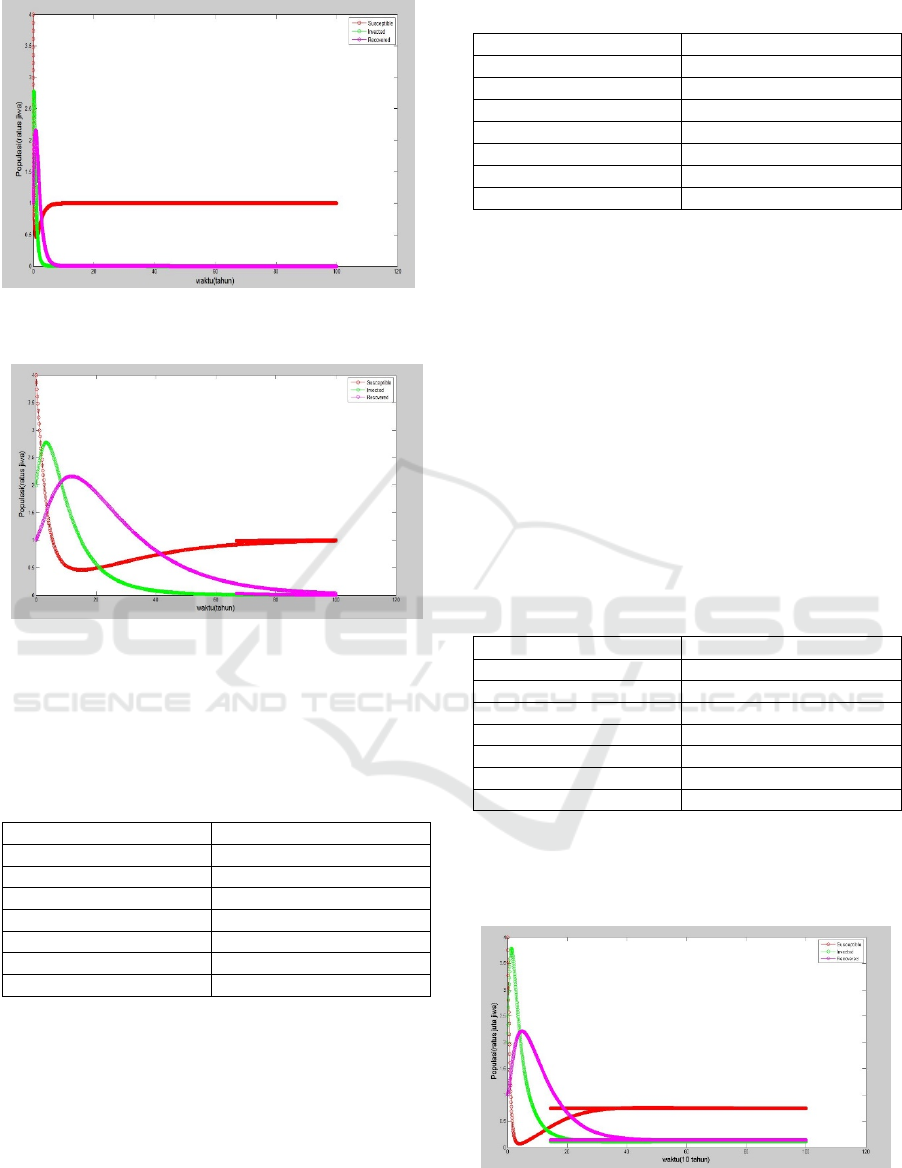
Figure 2: Simulation SIRS Model
1 with 0.01.
Figure 3: Simulation SIRS Model
1 with
0.09.
Table 3: The behavior of the system is based on the value
of
on the disease-free SIRS model.
Step time
System behavior
0,01 Stable
0,02 Stable
0,03 Stable
0,05 Stable
0,07 Stable
0,08 Stable
0,09 Unstable
The graph does not show stability in the
population because is so large, the graph will be
stable if the value is less than 0,09.
4.5.2 Simulation
1
For
1, given the parameter values to
qualify
1, from the values obtained value
1,34. The values are as follows:
Table 4: The parameter values simulation 1
1.
Parameter Value
0,012
0,026
0,008
0,006
0,002
0,0014
0,0017
From the initial values and given parameter
values
1 simulation is shown in Figure 4 and
5. The change in each population SIR against time,
population has decreased even close to zero. When
5 years, population has increased while
population and continue to decrease but not to
zero. This indicates that the epidemic disease will
become endemic.
The graph does not reflect system behavior over
time 0.07 as shown in Figure 6. So, it can be
concluded that the system is not stable at the time
range 0.07. The following present a table that
describes the stability of the system depends on the
value of .
Table 5: The behavior of the system is based on the value
of on the endemic SIRS model.
Step time
System behavior
0,01 Stable
0,02 Stable
0,03 Stable
0,04 Stable
0,05 Stable
0,06 Stable
0,07 Unstable
The graph does not show stability in the
population because h is large, the graph will be
stable if the value is less than 0,07.
Figure 4: Simulation 1 SIRS Model
1 with
0,01.
ICMR 2018 - International Conference on Multidisciplinary Research
82
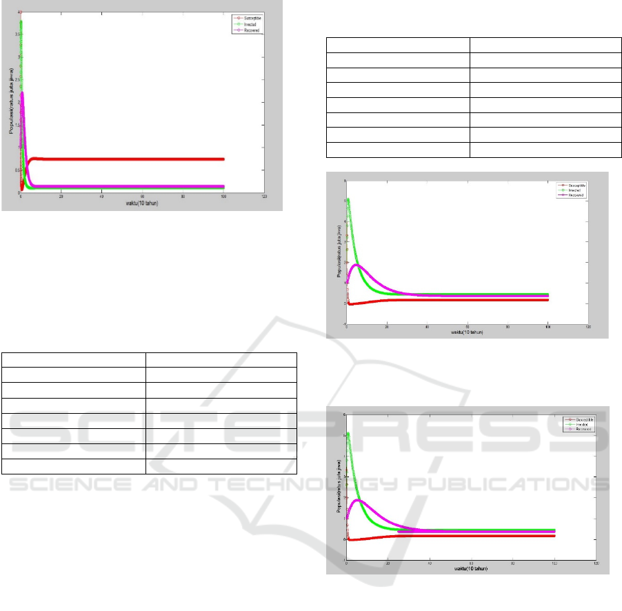
Figure 5: Simulation 1 SIRS Model
1 with
0,07.
Then given the values for simulation
1
with different parameter values, the values given are
as follows:
Table 6: The parameter values simulation 2
1.
Parameter Value
0,008
0,076
0,008
0,004
0,0016
0,0012
0,0017
From the initial value and the given parameter
values obtained simulation
1 shown in Figure
6 and 7. The population change of and is very
significant, population is at critical point while
population increases dramatically, population
also increase, but it does not affect population
because population increases very fast. When
10years population and decreased while
population increased but does not exceed
population as in figure 5.
The graph does not reflect the behavior of the
system at a time range 0.08 as in figure 7. The
following present a table that describes the stability
of the system depends on the value of .
Table 5: The behavior of the system is based on the value
of on the endemic SIRS model.
Step time
System behavior
0,01 Stable
0,02 Stable
0,03 Stable
0,04 Stable
0,05 Stable
0,06 Stable
0,07 Unstable
Figure 6: Simulation 2 SIRS Model
1 with
0,01.
Figure 7: Simulation 2 SIRS Model
1 with
0,07
.
The graph does not show stability in the
population because is so large, the graph will be
stable if the value is less than 0.08. So, the 5th
order Runge-Kutta numerical scheme satisfies the
stability properties of the SIRS model with
1
when the time step size is not greater than 0,07.
SIRS epidemic model simulation using Runge-
Kutta method of order 5 is influenced by time step
. The time step affects the time needed to
approach the equilibrium point, the greater the time
step is used the shorter the time needed to
approach the equilibrium point.
Stability Analysis of the SIRS Epidemic Model using the Fifth-order Runge Kutta Method
83

5 CONCLUSIONS
1) At condition
1 there is indication that the
behavior of the solution will be longer to point
, which means the longer the disease will be
lost from the population.
2) Under condition
1 there will be an
endemic condition, where the Infected
population is still in the population, in other
words the greater the rate of transmission of the
disease ( or the smaller the cure rate ( and
natural death causing endemic conditions.
3) Time step affects the time required to
approach the equilibrium point in the SIRS
epidemic model using the Runge-Kutta method
of order 5, the greater the time step
used
the shorter the time it takes to approach the
equilibrium point.
REFERENCES
Adda, P. & Bichara, D. 2012. Global Stability for SIR and
SIRS Models with Differential Mortality. International
Journal of Pure and Applied Mathematics. Vol. 80 No.
3 2012, 425-433.
Chapra, Steven C. 2004. Applied Numerical Methods with
MATLAB for Engineers and Scientists. Medford: The
McGraw-Hill Companies.
Marpaung, T.J., Tulus, dan Suwilo, S. 2018. Cooling
Optimization in Tubular Reactor of Palm Oil Waste
Processing. Bulletin of Mathematics Vol. 10, No. 01
(2018), pp. 13-24.
Sinuhaji, Ferdinand. 2015. “Model Epidemi SIRS dengan
Time Delay”. Jurnal Visipena. Vol. 6 No. 1 2015,78-
88.
Tulus. 2012. Numerical Study on the Stability of Takens-
Bogdanov systems. Bulletin of Mathematics. Vol. 04,
No. 01(2012), pp-17-24.
Tulus and Situmorang, M. 2017. Modeling of
Sedimentation Process in the Irrigation. Channel IOP
Conf. Series: Mat. Sci. Eng. 180 012021.
Tulus, Suriati and Situmorang, M. 2017. Computational
Analysis of Suspended Particles in the Irrigation.
Channel IOP Conf. Series: J. Phys. 801 012094.
Tulus, Suriati, and Marpaung T.J. 2018. Sedimentation
Optimitation on River Dam Flow by Using COMSOL
Multiphysics. Channel IOP Conf. Series: Mater, Sci.
Eng} 300 012051.
Tulus, Sitompul, O.S, Sawaluddin and Mardiningsih.
2015. Mathematical Modeling and Simulation of Fluid
Dynamic in Continuous Stirred Tank. Bulletin of
Mathematics Vol. 07, No. 02 (2015), pp. 1–12.
ICMR 2018 - International Conference on Multidisciplinary Research
84
