Investigation of Wave Orbital Velocity Estimation under

Non-breaking Irregular Waves

A. Haris Fattah, Suntoyo and Wahyudi

Department of Ocean Engineering, Faculty of Marine Technology, Institut Teknologi Sepuluh Nopember (ITS),

60111, Surabaya, Indonesia

Keywords: Wave Orbital Velocity, Irregular Wave, Bottom Shear Stress.

Abstract: Wave orbital velocity plays an important roles in many analysis of sediment transport calculation and

hydrodynamic model. The accuracy should be ensured to represent the actual conditions. This paper

reviewed and compared several approaches for estimating wave orbital velocity under non-breaking

irregular waves. There are four methods reviewed in this paper such as Stretching method, Local Fourier

Approximation (LFA) method, Fourier decomposition method, and a new proposed method based on the

Kaczmarek and Ostrowski (Kaczmarek and Ostrowski, 1996) by adding the correction coefficient factor (α

)

with value of 4.35. Those method has been examined and compared through both experimental data and the

estimation model. The proposed method gave the best agreement among other methods with smallest RMSE

value. The proposed method can be used to estimate wave orbital velocity under non-breaking irregular

waves with free surface elevation datas as an input in practical application.

1 INTRODUCTION

Wave orbital velocity plays an important roles in

many analysis of sediment transport and

hydrodynamics model in the case of coastal,

channel, and estuaries models. It should be ensured

that the estimation in accurate, so it can represent the

actual conditions in the field (Soulsby, 1987).

Time-varying of wave orbital velocities can be

calculated in several ways depending on the data

availability. Some researchers used spectrum

approach or wave by wave parameters. If measuring

devices (i.e. micro-ADV, LDV, or PIV) is available,

which is quite expensive tools for laboratory

equipment’s, then the wave orbital velocities can

obtained directly. It will be difficult when only the

wave surface elevation data obtained due to an

absence of measuring devices. Then the estimation

method for calculating the wave orbital velocity is

necessary.

The calculation methods of the wave orbital

velocity have been studied by many researchers, but

most of them are for regular and non-linear waves

e.g. (Sobey, 1992; Soulsby and Smallman, 1986;

Soulsby, 2006; Abreu et al., 2010; Suntoyo et al.,

2008; Suntoyo and Tanaka, 2009). However, it is

very rare to review wave orbital velocity for time

varying under non-breaking irregular wave’s

conditions. Several studies related to irregular waves

have been carried out by researchers (Soulsby, 1987;

Elfrink et al., 2006; Wiberg and Sherwood, 2008;

Malarkey and Davies, 2012; Suntoyo et al., 2016;

Wijaya et al., 2016; Fattah et al., 2018). However,

some of those methods have limitations on certain

conditions and a simple formulation due to non-

breaking irregular waves has not been proposed, yet.

Therefore, the objective of this study is to

examine and compare several formulation of wave

orbital velocity with experimental data under non-

breaking irregular waves motion (Ruiz, 2014). The

four calculation methods evaluated and exaimend

with a new proposed method based on the evaluation

of Fourier decomposition method (Kaczmarek and

Ostrowski, 1996), namely, Stretching method

(Wheeler, 1969), LFA method (Soulsby, 1987) and

Fourier decomposition (Kaczmarek and Ostrowski,

1996). The best agreement method obtained based

on the smallest value of RMSE (root-mean-squared-

error) as performance indicator. The best approach

will be further used to estimate the wave orbital

velocity under irregular wave motion.

200

Fattah, A., Suntoyo, . and Wahyudi, .

Investigation of Wave Orbital Velocity Estimation under Non-breaking Irregular Waves.

DOI: 10.5220/0008871202000204

In Proceedings of the 6th International Seminar on Ocean and Coastal Engineering, Environmental and Natural Disaster Management (ISOCEEN 2018), pages 200-204

ISBN: 978-989-758-455-8

2 WAVE PARAMETERIZATION

Wave orbital velocity can be calculated in several

ways depending on the available data. Some

common rules using wave by wave method or

spectrum parameterizations analysis to obtain wave

period and wave height from time series or spectra

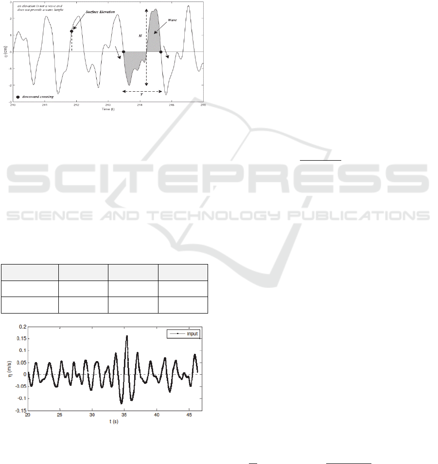
of surface elevation. In this present paper zero-down

crossing analysis method was used as as shown at

Figure 1 as given (Holthuijsen, 2007).

Figure 1: Definition of a “wave” with zero-down crossing

analysis in time records of surface elevation. (Holthuijsen,

2007).

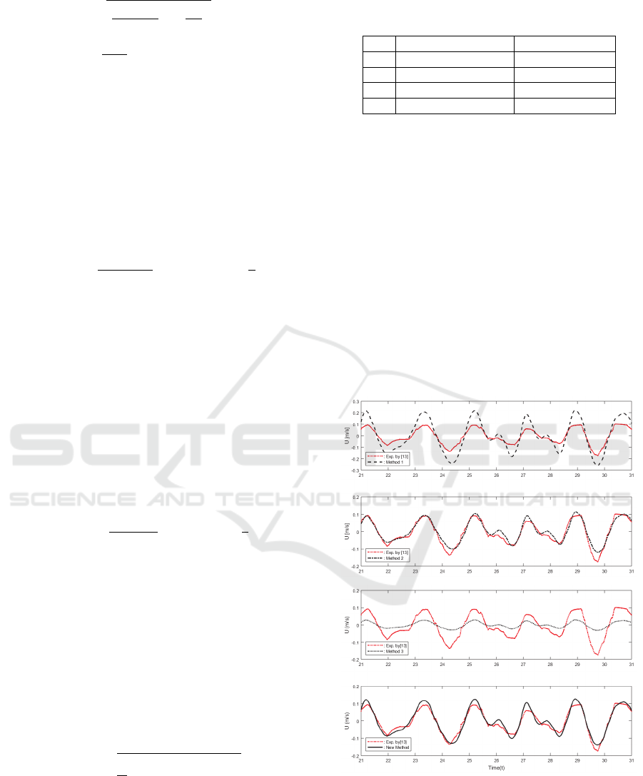
Surface-wave elevation and velocities data in this

paper was obtained by digitation from Ruiz (Ruiz,

2014) with totally 15 of wave cycles taken from 19s

until 48s of measured data. The velocity was

measured at z = -0.33 m with significant wave

height (Hs) = 0.14 m and wave peak period (Tp) =

1.98 s in 2.97m water depth as described in Table 1.

Table 1: Experimental data conditions (Ruiz, 2014).

ID Hs (m) Depth (m) Tp (s)

Plymouth A1 0.14 2.97 1.98

Plymooth B4 0.38 2.97 2.63

Figure 2: Surface wave elevation data Plymouth A1

obtained by digitation in Ruiz (Ruiz, 2014).

3 WAVE ORBITAL VELOCITY

CALCULATION METHODS

In this section, the four of existing wave orbital

velocity calculation methods under irregular waves

motion are presented. In this present paper, there are

four formula that evaluated and compared, namely,

Stretching method (Wheeler, 1969), LFA method

(Soulsby, 1987), Fourier decomposition (Kaczmarek

and Ostrowski, 1996) examined by a new proposed

method based on the evaluation of Fourier

decomposition method by Kaczmarek and

Ostrowski, (Kaczmarek and Ostrowski, 1996).

3.1 Method 1 (Stretching Method)

Wheeler (Wheeler, 1969) presented a method, the

so-called stretching method of Wheeler, which is

departed to calculate kinematic velocity from a

measured free surface time history (𝜂



𝑤𝑖𝑡ℎ 𝑖

1,2,…,𝐼 trough Airy kinematics solution. Then

transformed into Fourier-series transformation.

Therefore, the horizontal velocity is predicted as:

𝑢



𝐶



 𝑓𝜔



cosh𝛼



𝑘



ℎ

sinh𝑘



ℎ

𝜂





𝑡





/



𝑖1,2,… ,𝐼

(1)

𝜂



𝐴



cos



𝑓𝜔



𝑡



𝐵



sin



𝑓𝜔



𝑡



𝑓0,1,… ,𝐹/2

(2)

𝜂



 𝜂





𝑡





𝑖

/



1,2,…,𝐼

(3)

Where 𝐶



is Eulerian current (if current is

present), 𝛼



ℎ𝑧/ℎ𝜂



, 𝜔



2𝜋/𝑡





𝑡



 and 𝑘



is calculated from the linear dispersion

relation:

𝑔𝑘𝑡𝑎𝑛ℎ



𝑘ℎ



𝜔



0

(4)

3.2 Method 2 (Local Fourier

Approximation)

Local Fourier (LF) approximation is kinematics

calculation method presented by Soulsby (Soulsby,

1987) which addressed to calculate kinematics from

a measured free surface time-varying history by

means of a local approximation of the velocity

potential as a truncated Fourier series.

LF Approximation method based on an

approximation of the stream function (global) and

the velocity potential (local) as a truncated Fourier

series.

𝑢





𝜕𝜙

𝜕𝑥



𝑥,𝜂



,𝑡





𝐶







𝑗

𝑘𝐴



cosh

𝑗

𝑘



𝜂



ℎ



cosh 

𝑗

𝑘ℎ

cos 

𝑗

𝑘𝑥 





𝜔



𝑡





(5)

Investigation of Wave Orbital Velocity Estimation under Non-breaking Irregular Waves

201

𝐴











𝜕



𝜕



⁄



𝑘𝑡𝑎𝑛ℎ𝑘ℎ









𝑔𝜂



𝜔







(6)

𝐴





𝐴





𝑓𝑜𝑟

𝑗

1,…,𝐽

(7)

Where 𝜔



is estimated from the local zero-down

crossing period (𝑇



) as 𝜔



2𝜋/𝑇



3.3 Method 3 (Fourier Decomposition)

Kaczmarek and Ostrowski (Kaczmarek and

Ostrowski, 1996) proposed the simple method to

compute time series of wave orbital velocity based

on Fourier decomposition of the water surface

elevation as describes follow:

𝑈



𝑡



𝜂



𝜔



sinh 𝑘



ℎ

sin



𝜔



𝑡𝜑







𝑈





(8)

In which 𝜔



and 𝑘



are angular frequency and

wave number respectively, related to each other by

linear dispersion relationship. 𝜑



is phase and 𝑈



the average initial velocity.

3.4 Method 4 (Proposed Method)

A proposed method is simple method based on the

modification of Fourier decomposition method

(Kaczmarek and Ostrowski, 1996) by adding the

correction coefficient (α

) factor to the measurement

results of the experiment in the laboratory as

follows:

𝑈



𝑡



𝛼



𝜂



𝜔



sinh 𝑘



ℎ

sin



𝜔



𝑡𝜑







𝑈





(9)

In which 𝛼



is the correction coefficient with

value of 4.35.

4 RESULTS AND DISCUSSIONS

Evaluating the comparison of those different

methodologies presented above, it needs to be

validated using laboratory measurement data.

Comparison result evaluated trough the root-mean-

squared error (RMSE) defined as follow:

𝑅𝑀𝑆𝐸



𝑢







𝑁

𝑢





𝑢













(10)

Where, 𝑢





: the wave orbital velocity from

calculation methods, 𝑢





: the wave orbital velocity

from experimental results, N: total number of data

and i: index.

Table 2: Summary of calculation method performance of

wave orbital velocities.

No Method RMSE Value

1. Method 1 0.0668

2. Method 2 0.0289

3. Method 3 0.0791

4. Method 4 0.0265

If the calculation method is perfect, it can be

indicated that RMSE results should be zero. So, the

smaller RMSE is the better performance results of

the calculation methods. The summary of those

calculation method performance is presented in

Table-2.

Comparison results among the experimental data

and the calculation methods are given in Figure 2. It

can be seen that the proposed method (Method 4)

has highest performance with the lowest value of

RMSE among others methods with RMSE = 0.0265

then followed by Local Fourier (Method 2)

(Soulsby, 1987) with RMSE = 0.0307, Method

1(Wheeler, 1969) with RMSE=0.0668 and Method 3

(Kaczmarek and Ostrowski, 1996) with

RMSE=0.0781, respectively.

Figure 3: Comparison of the experimental data (Ruiz,

2014) and the calculation methods of wave orbital velocity

under non-breaking irregular waves.

Method 1 gives overestimation both in the crest

and trough of the waves, while Method 3 gives

significant different result against experimental data.

ISOCEEN 2018 - 6th International Seminar on Ocean and Coastal Engineering, Environmental and Natural Disaster Management

202

However, Method 3 is the simplest formula among

others while the Method 1 and Method 2 need

advance mathematical calculation to compute

approximation. Method 3 has a similar in line trend

with the experimental data, so it has an opportunity

to review further.

The proposed method (Method 4) that based on

the evaluation of the Method 3, with the addition of

a correction factor, gave smallest RMSE value

indicating that it has best agreement with the wave

orbital velocity of experimental result provided

(Ruiz, 2014). It can be concluded that Method 4 can

be used to estimate wave orbital velocities under

irregular waves with time-varying free surface

elevation as an input. Furthermore, the proposed

method can be further used to an input calculation of

bottom shear stress and sediment transport model

under non-breaking irregular waves in practical

application.

5 CONCLUSIONS

The calculation method of wave orbital velocity

under non-breaking irregular waves has been

examine and compare through both experimental

data and the estimation model. Method 4 as

proposed method gave best agreement with lowest

RMSE value and simplest formulation that

indicating the best performance among other method

then followed by Method 2, Method 1 and Method

3. Method 1 gave over estimation both in the crest

and trough condition of the waves. Method 3 gave

significant different results, but it has a similar in

line trend with the experimental data. Beside that,

Method 2 gave almost the same results with Method

4, but need an advance mathematical method to

estimate wave orbital velocity.Moreover, the

proposed method (Method 4) based on the

evaluation of the Method 3 by adding the correction

coefficient factor (α

) with value of 4.35 gave the

best agreement with the measured experimental data

than other estimation methods. It can be concluded

that proposed method can be used further to estimate

wave orbital velocity under non-breaking irregular

waves with free surface elevation data as an input in

practical application.

ACKNOWLEDGEMENTS

The first author is grateful for the supported by

Higher-Education, Ministry of Research and

Technology and Higher Education RI, LPPM-ITS,

Institut Teknologi Sepuluh Nopember (ITS)

Surabaya, Indonesia. This research was partially

supported by PMDSU Research Program (No:

135/SP2H/LT/DRPM/2018)

REFERENCES

Abreu, T., Silva, P. A., Sancho, F., and Temperville, A.,

2010. Analytical approximate wave form for

asymmetric waves. Coastal Engineering 57 (7) : 656-

667.

Elfrink, B., Hanes, D. M., and Ruessink, B. G. 2006.

Parameterization and simulation of near bed orbital

velocities under irregular waves in shallow water.

Coastal Engineering 53 (11) : 915-927.

Fattah, A.H., Suntoyo, and Damerianne, H.A. , 2018.

Hydrodynamics and Sediment Transport Modelling of

Suralaya Coastal Area, Cilegon, Indonesia. IOP Conf.

Series : Earth and Environmental Science 135:

012024.

Holthuijsen L.H, 2007. Waves in Oceanic and Coastal

Waters. UK. Cambridge University Press.

Kaczmarek, L.M., and Ostrowski, R., 1996. Asymmetric

and Irregular Wave Effects on Bedload: Theory versus

Laboratory and Field Experiments. Proceedings of

25th Conference on Coastal Engineering, Orlando,

Florida.

Malarkey, J., and Davies, A. G. 2012. Free stream velocity

descriptions under waves with skewness and

asymmetry. Coastal Engineering 68 (2012) : 78-95.

Ruiz, P.M., 2014. Methods for prediction of wave

kinematics. MSc Thesis, School of Engineering and

Science. Aalborg University, Denmark.

Sobey, R. J., 1992. A local Fourier approximation method

for irregular wave kinematics. Applied Ocean

Research, 14: 93-105.

Soulsby and Smallman, 1986. A direct method of

calculating bottom orbital velocity under waves.

Hydraulics Research. Wallingford. Report number

SR-76 (36).

Soulsby, R.L. 1987. Calculating bottom orbital velocity

beneath waves. Coastal Engineering 11(4) :371-380

Soulsby,R.L., 2006. Simplified calculation of wave orbital

velocities. HR Wallingfor Report (TR 155)

Suntoyo, Tanaka H., and Sana A., 2008. Characteristics of

turbulent boundary layers over a rough bed under saw-

tooth waves and its application to sediment transport.

Coastal Engineering 55 (12): 1102-1112.

Suntoyo, and Tanaka H., 2009. Effect of bed roughness on

turbulent boundary layer and net sediment transport

under asymmetric waves. Coastal Engineering 56 (9):

960-969.

Suntoyo, Fattah A.H., Fahmi M.Y., Rachman T., and

Tanaka H., 2016 Bottom shear stress and bed load

sediment transport due to irregular wave

motion, ARPN Journal of Engineering and Applied

Sciences 11(2): 825-829.

Investigation of Wave Orbital Velocity Estimation under Non-breaking Irregular Waves

203

Wheeler,J.D., Method for calculating forces produced by

irregular waves. Proc. 1

Annual Offshore Technology

Conference, Houston, 1 (1696) 71-82.

Wiberg, P., and Sherwood, C. 2008. Calculating wave-

generated bottom orbital velocities from surface-wave

parameters. Computers and Geosciences 34 (10) :

1243-1262.

Wijaya, M. M., Suntoyo, and Damerianne, H. A., 2016.

Bottom shear stress and bed load sediment transport

formula for modeling the morphological change in the

canal water intake. ARPN Journal of Engineering and

Applied Sciences 11(4): 2723-2728.

ISOCEEN 2018 - 6th International Seminar on Ocean and Coastal Engineering, Environmental and Natural Disaster Management

204