Estimation of River Flood Discharge by using 2D Model

Akbar Rizaldi

, Idham Riyando Moe

, Mohammad Farid

and Herryan Kendra

Center for Water Resources Development, Institute for Research and Community Services, Institut Teknologi Bandung,

Jalan Ganesha No.10, Bandung 40132, Indonesia

Directorate General of Water Resources, Ministry of Public Works and Housing,

Jalan Pattimura No. 20, Kebayoran Baru, Jakarta Selatan 12110, Indonesia

Water Resources Engineering Research Group, Institut Teknologi Bandung,

Jalan Ganesha No.10, Bandung 40132, Indonesia

Aditya Engineering Consultant, Jl. Batu Permata 1 No. 2A Margacinta, Bandung 40286, Indonesia

Keywords: River Flood, Discharge, 2D Model.

Abstract: Flood disaster is still a problem in many countries in the world; therefore, it is also still important to study

about the flood. There have been many flood studies conducted by researchers. Modelling is one of the topics

of flood studies which is usually discussed. Two-dimensional (2D) model is commonly used in flood

modelling because it provides more information compared with one dimensional (1D) model. By doing flood

simulation using a 2D model, important information, particularly related to inundation area, can be obtained

so that the analysis in the flood study can be more comprehensive. In this study, 2D flood model is applied to

Bolango River in order to estimate its actual capacity. The modelling process is conducted by using rainfall

ground stations in a period of 2010-2017, land-use map data in 2015, and a digital elevation model (DEM) by

combining SRTM data and observed cross-section data. The boundary condition at the downstream is sea

water level and at the upstream is the flood discharge from Bone River. The model is verified by comparing

inundated area from simulation result with the observation data. The model result shows good agreement with

the observed data. Based on the result, the bank-full capacity of Bolango River is 189 m3/s, which is just 30%

of 25 years return period of flood discharge.

1 INTRODUCTION

River flood modelling is a tool for assessment,

evaluation, and prediction of river flood risk in

various scenarios (Alaghmand, et.al, 2012).

Hydraulic modelling can certainly provide reliable

and accurate results especially when the model can

exploit the extensive information provided nowadays

(Detrembleur, et.al, 2009). Not only extensive, the

information needed must be accurate and up-to-date.

Thus, the flood rapid assessment is very important to

provide a better accurate hydraulic or flood model

(Moe, et.al, 2018). There are many flood modelling

software was developed to help engineers design,

assess, and evaluate drainage system and provide

them to analyse it in 1-D, 2-D, and 3-Dimensional

model. 2D modelling is considered as a model that

has a better accuracy rate than the 1D modelling

(Gharbi, et.al, 2016; Yakti, et.al, 2018). And also, 2D

model has been considered as the best way to simulate

flood inundation due to its effectiveness and

efficiency (Farid, et.al, 2017). Several considerations

should be done to decide which model will be used in

the study, such as the complexity of river scheme, the

flow characteristic, the availability of observation

data, until the capacity of hardware that will be used

in flood modelling.

Flood is one of the most common natural disasters

in Indonesia. Likewise, the city of Gorontalo which

crossed by the Bolango River. The Bolango River has

experience with flooding almost every year and it is

more frequent in the last five years, such as in 2002,

2013, 2014, 2016, and 2017. This incident causes

harm not only to the material but also to the victims.

Flood on the Bolango River is caused by several

causes such as land-use changes due to the

urbanization, small river capacity, high sedimentation

accumulation, and climate change also contributed to

the causes of the flood in the Bolango River.

Several studies have been conducted to deal with

or to reduce the flood in Gorontalo City. Lihawa and

Rizaldi, A., Moe, I., Farid, M. and Kendra, H.

Estimation of River Flood Discharge by using 2D Model.

DOI: 10.5220/0008560301370143

In Proceedings of the 6th International Seminar on Ocean and Coastal Engineering, Environmental and Natural Disaster Management (ISOCEEN 2018), pages 137-143

ISBN: 978-989-758-455-8

137

Sutikno (2009) also reported that the problem of

sedimentation was one of the causes of the flood in

Gorontalo City . In 2012, Arifin et al. have conducted

research on flood disaster risk maps based on several

factors such as rainfall, geological conditions, soil

type, groundwater table, topography and land cover.

Then in 2014, Sarwono et al. had done the assessment

of flood in the Province of Gorontalo to know the

conditions of the drainage system, hydrological

condition, and the rivers morphology. Utama et al. in

2015 reported that the Bolango River had large

sedimentation problems which had a large impact on

flooding. The aim of this study is utilizing the 2-

dimensional flood model to analyse Bolango river

capacity.

2 GOVERNING EQUATIONS

There are three types of approach models can be used

in flood modelling, one-dimensional, two-

dimensional, and three-dimensional. A one-

dimensional model is only considered flow in one

dimension (one-axis flow). Two and three-

dimensional modelling allows the numerical

simulation to expanse the flow from the river into

others axis respectively (Paudel, et.al, 2016; DHI,

2017).

2.1 One-dimensional Hydraulic Model

The equations are used in the numerical model is the

Saint Venant equations. The Saint Venant Equations

is consist of the continuity and the momentum

equations as given below.

Continuity









(1)

Momentum



























QgQn



( 2 )

Where Q is discharge (m3 s-1), A is cross-

sectional area (m2), q1 is a distributed lateral inflow

or outflow along the x-axis from watercourse (m2 s-

1), n is Manning's roughness coefficient, α is

momentum distribution coefficient, g is acceleration

of gravity (m s-2), R is hydraulic radius (m), and h is

water level (m).

2.2 Two-dimensional Hydraulic Model

In the two-dimensional model, the equations are used

in the calculation process is same, St. Venant

equation. But, the equation will be derived into 2-

dimensional form to calculate flow characteristics in

2-dimensional. The Saint Venant equations are

written in the following form:

0











(3)







































































)(

qpgp







(4)



































































)(

xyyy

yhC

qpgq







(5)

Where x and y are the horizontal Cartesian

coordinates; h is the water depth; C(x,y) is Chézy

resistance (m1/2 s-1); ζ(x,y,t) is the water surface

elevation (m); g is the gravitational acceleration; ρw

is the density of water; τxy, τxx and τyy are the depth-

averaged turbulent stresses (kg m-1 s-2), and p(x,y,t),

q(x,y,t) are flux densities (m3 s-1 m-1) in x- and y-

directions.

2.3 Rainfall Run-off Model

The rainfall run-off model is used in this study is

lumped-sum rainfall run-off model by Nakayasu

model. This model is generated based on observations

of several rivers in Japan. The peak discharge can be

calculated by using the equation following:

𝑄









,,





,



(6)

Where C is the run-off coefficient from land use

of basin; Qp is the peak discharge (m3/s); R0 is the

unit rainfall (mm); A is the area of basin (km2), Tp is

the time of rain starts to peak discharge (hours); T0,3

the time needed for discharge decreasing to 30% of

the peak (hours)

trtgTp 8,0





(7)

tgtr 5,0



(8)

Time concentration can be calculated follows:

For L < 15 km

ISOCEEN 2018 - 6th International Seminar on Ocean and Coastal Engineering, Environmental and Natural Disaster Management

138

7,0

21,0 Ltg 

(9)

For L ≥ 15 km

Ltg 058,04,0 

(10)

Where tg is the time of concentration (hour); tr is

the effective time(hour); and L is the length of river

(km). The time needed to reduce the discharge from

peak discharge to 30% of peak discharge can be

calculated follow:

tgt .

3,0





(11)





25,0

47,0





(12)

Where α is the runoff coefficient. α = 2; for regular

basin, α = 1,5; for the rising part the hydrograph is

slow and falls rapidly, and α = 3; for the hydrograph

rises rapidly and falls slowly.

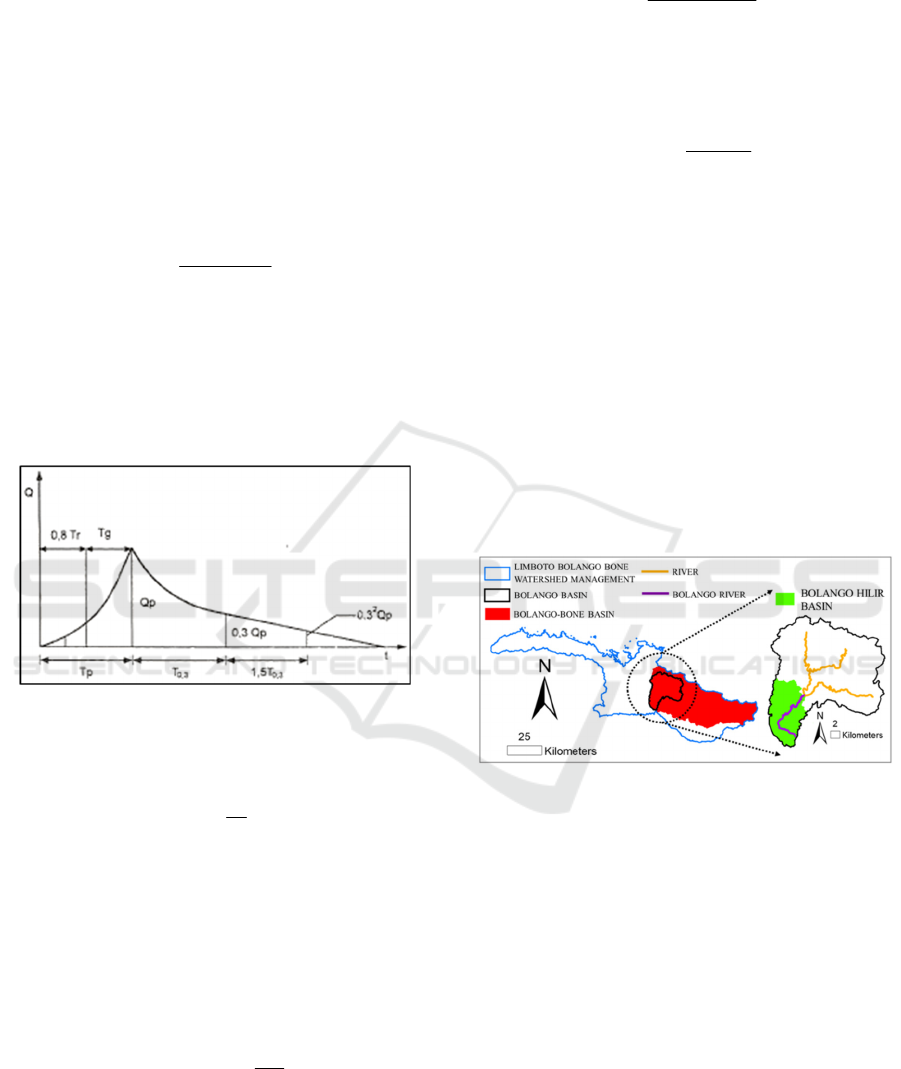
To make a hydrograph there is a rule to make

hydrograph like a Nakayasu hydrograph shape (see

Figure 1).

Figure 1: Nakayasu Hydrograph.

Unit hydrograph curves / rising limbs have the

following equation:

4,2















QpQa

(13)

𝑇  𝑇𝑝

Where Qa is run-off before reaching peak

discharge (m3/s); T is time (hour); Qp is peak

discharge (m3/s), and Tp is time peak (hours).

The decreasing limb has the following equation:

Curve down 1:

Tp ≤ t ≤ Tp + T

0,3



3,0

3,0.1

Tpt

QpQd





(14)

Curve down 2:

Tp + T0,3 ≤ t ≤ Tp + 1,5T0,3

3,0

5,1

3,0

5,0

3,0.2

TTpt

QpQd

















(15)

Curve down 3:

Tp + 1,5T0,3 ≤ t



3,0

5,1

3,0.3

TTpt

QpQd





(16)

3 DESCRIPTION OF THE STUDY

AREA

This paper studies the use of 2-dimensional flood

modelling to assess the capacity of Bolango River.

The river flow through Gorontalo City (the south of

Gorontalo). The Bolango Basin has an area of 398

km2, with the longest river in that basin is Bolango

River. The length of Bolango river from upstream to

downstream is around 17 km. the main section of this

study, which is the river section to be observed in this

study is the downstream section (Pink line on Figure

2) which have a contact with Gorontalo City.

Figure 2: Bolango River Basin Location.

4 MATERIALS AND METHODS

4.1 Elevation Data

The elevation data used in this study comes from the

National Aeronautics and Space Administration

(NASA) from the United States. The elevation data

used in this study has a level of 30 meters resolution.

From the elevation data, it is known that the

downstream area (Gorontalo City) has a flat height

with an elevation of about 1 to 8 meters above the

mean sea level (Mean Sea Level). This situation can

be seen in Figure 3. While the situation in the

mountains has a very high and steep slope between

1300-1500 m above the average surface of sea water.

Estimation of River Flood Discharge by using 2D Model

139

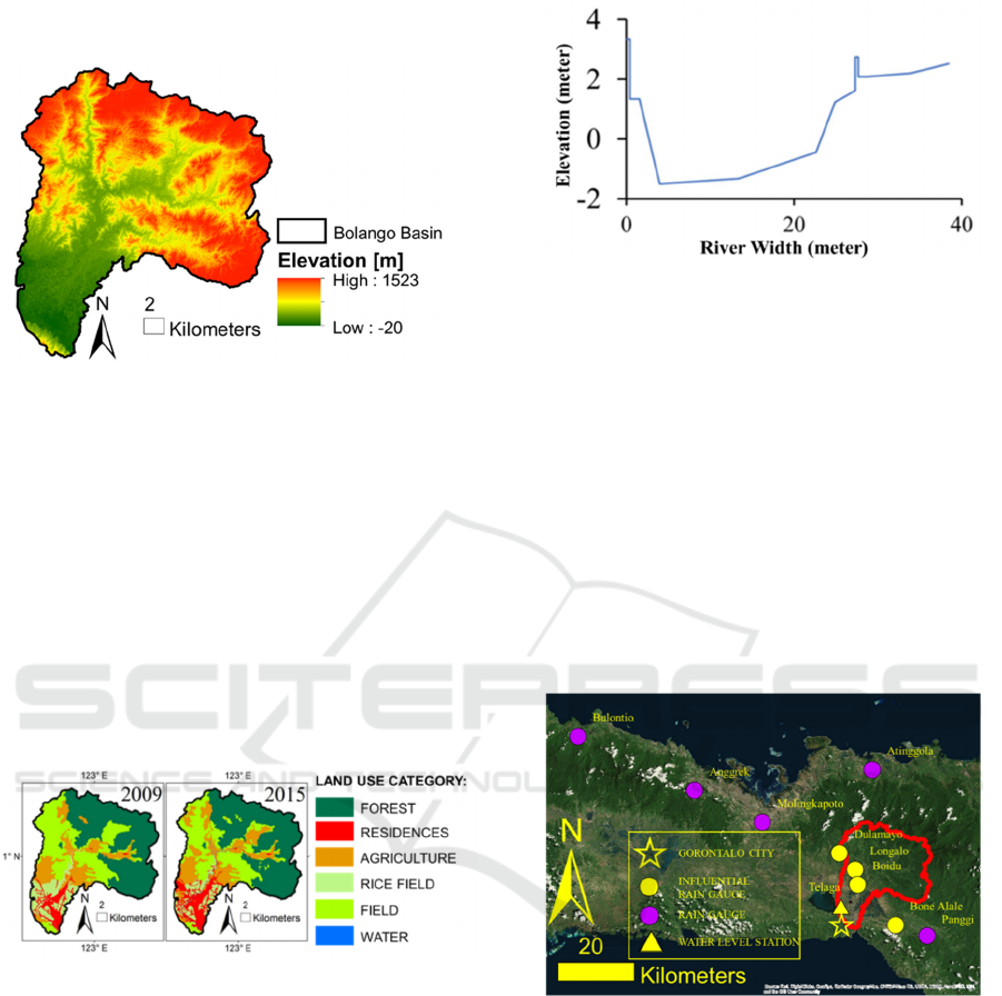
The mountainous altitude situation in the upstream

city of Gorontalo can also be seen in Figure 3.

Figure 3: Elevation Data of Bolango Basin.

4.2 Land Use Data

The Gorontalo City is filled with shops and

government centres as shown in Figure 4 below,

where land use is filled with urban areas in 2015. It

can be seen also in Figure 4 that the state of land use

in the upstream part of Gorontalo is still a forest area

and open land both in 2009 and 2015. However,

changes in land use from rice fields or open land to

urban areas will have a great opportunity to occur as

shown in Figure 4. This also means that the situation

of increasing urbanization will still be possible in the

future.

Figure 4: Land use Change.

4.3 Cross-section Data

The cross-section data used in this study is data

derived from the study of Balai Besar Wilayah Sungai

Sulawesi II. In Figure 5 below, is an example of a

cross section measured by the BWS Sulawesi II

Team. This cross-section data will be used as the

initial initiation input for the inundation flood model

to find out the parts that can be passed by the water in

this downstream Bolango River.

Figure 5: Example of Cross Section Bolango River.

4.4 Rain Gauge Data

Based on the spatial analysis of rain gauges from 9

stations, there are only 4 stations that have an

influence on the Bolago River Basin, namely Alale

Station, Longalo Station, Dulamayo Station, and

Boidu Bolango Station. So that the rain gauge is used

as a frequency analysis of the return period (Tr).

There are 4 out of 9 rain gauge with a daily

temporal distribution on the target area that has a

series of rain data that is quite good and uniform.

Namely Dulamayo, Longalo, Boidu, and Alale. Also,

there is a water level station (see Figure 6) to calibrate

the rainfall-runoff model.

Figure 6: Rain Gauge and Water Level Station.

The calculation of the return period of rainfall

based on the average area of rainfall data in Bolango

Basin. The maximum daily rainfall from each year

can be seen in Table 1.

ISOCEEN 2018 - 6th International Seminar on Ocean and Coastal Engineering, Environmental and Natural Disaster Management

140

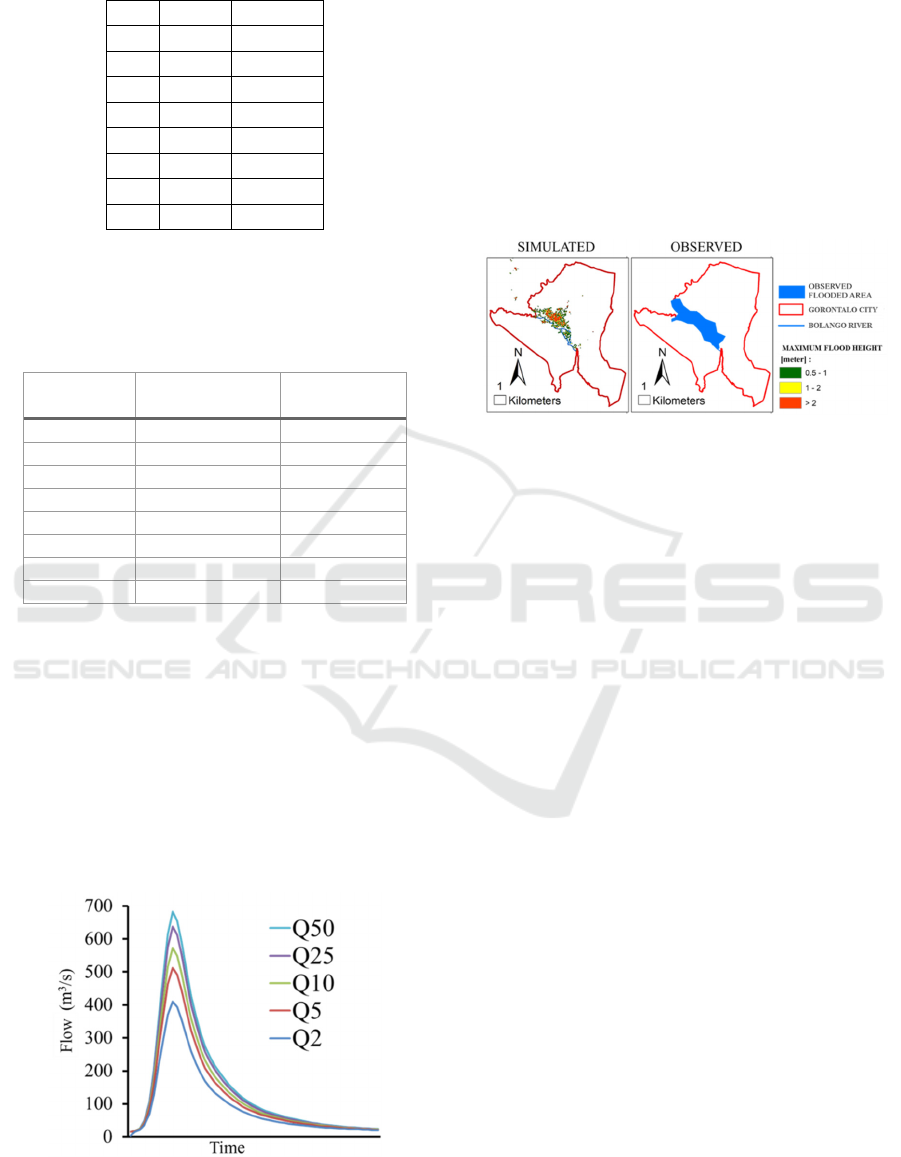
Table 1: Maximum Rainfall Data.

No Years R

Max

1 2010 55.7

2 2011 47.8

3 2012 57.8

4 2013 52.4

5 2014 65.7

6 2015 52.7

7 2016 76.6

8 2017 62.4

Then the rain calculation is done again using the

Gumbel distribution. From the calculations that have

been made, the following values are generated.

Table 2: Return Period of Rain.

Return

Period

Probability Rainfall (mm)

2 0.5 57

5 0.8 69

10 0.9 76

25 0.96 86

50 0.98 93

100 0.99 100

200 0.995 107

1000 0.999 123

4.5 Flow Data

Flow data were generated by Nakayasu rainfall-

runoff model as described in the previous section. The

relationship of rainfall and flow recorded in the

calculation of the amount of discharge that affects the

flooded unit in the study area. The flow hydrograph

was calculated after the Nakayasu model was

calibrated by observation data at Talaga Water Level

Station. The calculated hydrograph flow can be seen

in Figure 7

Figure 7: Flow Hydrograph.

5 SIMULATION AND RESULT

We use the 1-D hydraulic model, then coupling it

with a 2-D model to do flood simulation. Before we

do flood simulation we should calibrate the flood

model with observation data. This is the important

stage because to get the exact capacity of Bolango

River we should make sure that the model we will use

in flood modelling represents the actual condition of

the river. Then we do the calibration process and we

can see the result follow Figure 8.

Figure 8: Calibration Result.

Figure 8 (left) the result of a simulation of

inundation floods due to flooding on the Bolango

River with Q25. The left one is the simulated flood

situation with Q25 using the measurement data of the

original cross section. The right picture is the most

disaster-prone zone map. This map of disaster-prone

zones comes from Arifin et al (2016). We can see that

the comparison between simulation and observation

has a fairly close relationship. We get some calibrated

parameters data, Manning's roughness coefficient (n)

for river bed is 0,03 – 0,6 and for floodplain,

Manning's roughness coefficient (n) is around 0,4.

That is, this flood model is quite well calibrated.

After the calibration process, the current capacity

of the Bolango River bankfull can be evaluated. For

the information, the results of the model calibration in

this study use a return period flow (Q25). Then, we

carried out several numerical simulation scenarios to

testing the inundation flood model by using Q25 as

input for the model. This scenario is to reduce the Q25

discharge by 0.7 times, 0.5 times, 0.32 times, 0.31

times and 0.3 times. The graph of each discharge

scenario can be seen in Figure 9. Each scenario will

be numerically tested using a flood inundation model.

Estimation of River Flood Discharge by using 2D Model

141

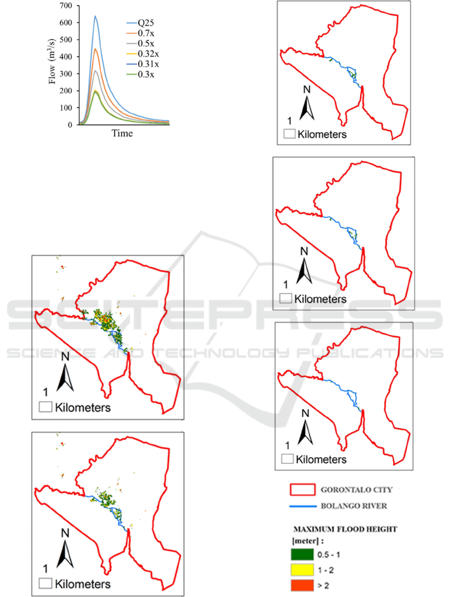
Figure 9: Flow Scenario to Evaluate the river capacity.

The flow hydrograph from each scenario are used

as input for the inundation flood model. Inundation

flood situation of each discharge scenario in Figure 9

can be seen from the inundation simulation results in

Figure 10. For the record, the simulation of

inundation results presented is the maximum

inundation height in each simulation scenario.

(i)

(ii)

(iii)

(iv)

(v)

Figure 10: Flood Simulation Results: (i) 0,7 X ; (ii) 0,5 X ;

(iii) 0,32 X ;(iv) 0,31 X ; and (v) 0,3 X.

ISOCEEN 2018 - 6th International Seminar on Ocean and Coastal Engineering, Environmental and Natural Disaster Management

142

From Figure 10 above we can see that with a

discharge scenario of 0.3 from Q25 there is hardly

any more inundation in the target area of the study

area. That is, from the results of numerical

simulations carried out, peak discharge with 189 m3/s

is a bankfull capacity for the current Bolango River.

This also means that bankfull capacity for the

Bolango River is 30% of Q25. And that is below the

value of flow with a return period 2-year. This

bankfull capacity might decrease when the

accumulation of sedimentation in the Bolango River

increases following the time.

6 CONCLUSION

In this study, the inundation floods model of Bolango

River was constructed. Simulation results of flood

inundation from the flood inundation model have

been compared with inundation observations data and

have a fairly close relationship between the two. From

that conclusion, the model has been calibrated and

can be used to produce a flood inundation simulation.

Based on the results of numerical simulations, the

average maximum peak discharge capacity of the

Bolango River downstream is 189 m3/s. This peak

discharge situation is 30% of the Q25 return period

flow. That is the amount of discharge that can be

drained by the Bolango River without any inundated

area along the river. The situation of the maximum

discharge that can be traversed by the water in the

downstream Bolango River will become smaller in

capacity when considering the accumulation of

sedimentation that might increase in the future.

REFERENCES

B. P. Yakti, M. B. Adityawan, M. Farid, Y. Suryadi, J.

Nugroho, and I. K. Hadihardaja, 2018. MATEC Web of

Conferences, 147, 03009.

B. Sarwono, Sutikno, U. Lasminto, K. A. Utama, and A.

Zainuri, 2014. Prosiding Seminar Nasional Aplikasi

Teknologi Prasarana Wilayah (ATPW), ISSN 2301-

6752.

DHI, 2017. MIKE 21 & MIKE 3 Flow Model FM

Hydrodynamic and Transport Module Scientific

Documentation, MIKE DHI.

F. Lihawa and Sutikno, 2009. IJG Vol. 41 No. 2, 103-122,

ISSN 0024-9521.

I. Arifin Yayu and M. Kasim, 2012. Program Studi

Geografi Fakultas Matematika dan IPA, Universitas

Negeri Gorontalo.

I. R. Moe, A. Rizaldi, M. Farid, A. S. Moerwanto, and A.

A. Kuntoro, 2018. MATEC Web of Conferences, 229,

04011.

K. A. Utama and R. Husnan, 2015. Fakultas Teknik

Universitas Negeri Gorontalo.

M. Farid, A. Marlina, and M. S. B. Kusuma, 2017. AIP

Conference Proceedings, vol. 1903(1), 100009.

M. Gharbi, A. Soualmia, D. Dartus, and L. Masbernat,

2016. J. Mater. Environ. Sci., 7 (8), 3017-3026.

M. Paudel, S. B. Roman, and J. Prichard, 2016. Wood

Rodger Inc., Sacramento, CA.

S. Alaghmand, R. Abdullah, and I. Abustan, 2012. Int. J.

Hydrology Science and Technology, Vol. 2, No. 3.

S. Detrembleur, B. J. Dewals, P. Archambeau, S. Erpicum,

and A. Pirotton, 2009. Associ. Sci. Tech. Eau. Environ.

7, 23-29.

Estimation of River Flood Discharge by using 2D Model

143