Numerical Study on Inﬂuence of Hydrofoil Clearance towards Total

Drag Reduction on Winged Air Induction Pipe for Air Lubrication

Yanuar

∗

,Muhammad Akbar

, M. Alief

, Fatimatuzzahra

, and Made

Department of Mechanical Engineering, University of Indonesia, Depok, Indonesia

Keywords:

Drag Reduction, Air Lubrication, Hydrofoil, Multi-Phase Flow, Computational Fluid Dynamics.

Abstract:

A new device for air lubrication called Winged Air Induction Pipe (WAIP) is studied in the present work.

The device, which consists of angled hydrofoil uses the low-pressure region produced above the hydrofoil as

ship moves forward. The low pressure drives the atmospheric air into the water in certain velocities which the

pressure is negative compare to atmospheric pressure. A computational ﬂuid dynamics approach is presented

to study the effect of hydrofoil clearance of Winged Air Induction Pipe in drag reduction experienced by the

plate which WAIP attached. The well-known ’volume of ﬂuid’ model and k-ω SST (shear stress transport)

turbulence closure model have been used in the 2D numerical simulation in ANSYS Fluent. The numerical

simulation is carried out with different conﬁguration of hydrofoil clearance and angle of attack. Effects of

these parameters on total drag force and drag reduction are reported. The reduction of drag force is found to

increase to about 10% compared to bare plate conﬁguration.

1 INTRODUCTION

The methods of drag reduction using air lubrication

are becoming promising study due to the increase

of fuel efﬁciency produced as the result of reduced

drag(Cui et al., 2003). The principle of air lubrica-

tion method is to reduce the Reynold shear stress oc-

curs on the boundary layer of the ﬂow (Yanuar et al.,

2012)(Toffoli et al., 2010). The magnitudes of the

Reynold shear stress can be moderately changed by

the dispersed phase for the dilute two-phase ﬂow, but

the distribution pattern keeps unchanged (Muste et al.,

2009). Kodama et al. (2000) found promising result

using air lubrication in the form of microbubble for

drag reduction. It is well known that the presence

of the air in the turbulent boundary layer of the ﬂow

leads to drag reduction for two reasons: ﬁrst by low-

ering the average viscosity and density of the mixture

ﬂow. The mixture of gas and liquid has lower density

and viscosity compare to the liquid itself; second, by

decreasing the magnitudes of the Reynold shear stress

through the interaction of the air and liquid.

Numerical study also can be performed to calcu-

late drag reduction produced by air lubrication. Nu-

merical study has been done as an alternative to ex-

perimental study as the numerical requires less time

and still gives accurate result by conducting valida-

tion towards the similar experimental result ﬁrst. Var-

ious numerical study has been performed to calculate

the drag reduction using various air lubrication. Mo-

hanarangam et al. (2009) studied the phenomenon of

drag reduction by the drag reduction by the injection

of microbubble into a turbulent boundary layer us-

ing a Eulerian–Eulerian two-ﬂuid model. Pang et al.

(2014) investigated microbubble drag reduction using

the Euler–Lagrange two-way coupling method in or-

der to understand the drag reduction mechanism by

microbubbles. Shereena et al. (2013)) and Evans et al.

(1992) conducted a numerical simulation using k-ω

SST to calculate the drag reduction produced by air

jet on an axisymmetric underwater vehicle.

The air lubrication requires an injection to dis-

perse air into the water. The injection requires en-

ergy due to the higher pressure in the water partic-

ularly in certain depth in the ship bottom hull. The

pressure from air compressor is required in order to

inject air into the water. However, the amount of en-

ergy required is large enough to cancel out a part of

the energy saved by the air lubrication. The injection

of the air into the water in certain depth requires vari-

ous source of energy: ﬁrst the adiabatic compression,

the air generation in the water and mechanical losses

at the air compressor (Kumagai et al., 2015). As the

result, he net-power saving declines as little as 5%.

Kumagai et al. (2015) found a new device called

Winged Air Induction Pipe (WAIP). The WAIP con-

Yanuar, ., Akbar, M., Alief, M., , F. and , M.

Numerical Study on Inﬂuence of Hydrofoil Clearance towards Total Drag Reduction on Winged Air Induction Pipe for Air Lubrication.

DOI: 10.5220/0008544001630169

In Proceedings of the 3rd International Conference on Marine Technology (SENTA 2018), pages 163-169

ISBN: 978-989-758-436-7

163

sist of the air pipe and angled hydrofoil that has a

lower pressure in the upper surface due to the higher

velocity magnitudes. Previously, numerous studies on

the effect of the hydrofoil on air-water interface has

been performed. Duncan (1981) conducted and ex-

periment of the breaking waves produces by a towed

hydrofoil at constant depth and velocity. Kumagai

et al. (2011) and Muratoglu and Yuce (2015) found

that the hydrofoil also produces a negative pressure

that pull in the air above into the water as the hydro-

foil positioned near the water surface.

In the present work the WAIP from previous work

(Kumagai et al., 2015) is studied. The device pro-

duces natural air injection without using an air com-

pressor at critical velocity Uc that is deﬁned as:

2gHα

α − (L/h

sinθ

(1)

where g is gravity acceleration, H is the depth of the

injection, α is the mean void fraction, C

is pressure

coefﬁcient, and L, h

, C

, and θ are hydrofoil chord

length, the air-water mixture layer thickness, and hy-

drofoil angle of attack respectively. However, in their

study Kumagai et al. (2015) found that the hydrofoil

in some cases develop some problem regarding the

clearance to the bottom plate where the WAIP placed.

Additionally, it should be noticed that the present nu-

merical simulation is aimed to analyze the inﬂuence

of the hydrofoil clearance in Winged Air Induction

Pipe towards the amount of drag reduction produced

and the relationship between the angle of attack and

clearance of the hydrofoil in WAIP device.

2 NUMERICAL STRATEGIES

For simulating two phase ﬂow, the Volume of Fluid

(VOF), as implemented in Fluent, is used. This can

be used to model the separation of air and water above

and below the ship respectively. The water is imple-

mented as the primary phase and air as the secondary

phase. The surface tension modeling also used in the

modeling to achieve representation of the air-water

contour. For a best viewing experience the used font

must be Times New Roman, on a Macintosh use the

font named times, except on special occasions, such

as program code (Section 2.3.7).

2.1 Governing Equations

Three dimensional, transient, viscous, incompress-

ible, and two-phase immiscible ﬂuid ﬂow is numer-

ically solved by discretizing RANS equations.

∇ · U = 0 (2)

Figure 1: Schematic diagram from side-view of the compu-

tational setup

δρU

δt

+ ∇(ρUU

) = −∇p

∗

+ ∇(µ∇U) + ∇(ρτ) + S

(3)

where U = (u

+ u

) is the velocity vector, t

is time. ∇ is vector differential. p∗ is relative pres-

sure. ρ and µ are ﬂuid properties the density and dy-

namic viscosity, respectively τ is Reynold stress ten-

sor for turbulence ﬂow. Closure of the turbulence

model for τ is k-ω Shear Stress Transport (SST). The

turbulence kinetic energy k and speciﬁc dissipation

rate ω are estimated from the boundary condition of

turbulence quantities turbulence intensity I and length

scale l. For simulating turbulent ﬂow, the Shear-Stress

Transport (SST) k-ω is used to model the near wall

region of the ﬂow. This is based on previous study

that found this model is well suited for simulating

two phase ﬂows(Mohanarangam et al., 2009). The

k-ω SST model is an effective blend of robust and ac-

curate formulation of the k-ω in the near wall region

and k-ω model in the far ﬁeld (Shereena et al., 2013).

The k-ω SST model gives more realistic result in pre-

diction of void fraction occurs in the near wall region

(Menter, 1994). Instead of using empirical wall func-

tion to correlate the near wall and far ﬁeld region, k-ω

SST solved two turbulence scalar directly towards the

wall boundary (Mohanarangam et al., 2009). SST k-ω

can be described as: Kinematic eddy viscosity

max(a

ωSF

)

(4)

Turbulent kinetic energy

δk

δt

δk

δx

= P

− β

∗

kωt +

δx



(ν + σ

)

δk

δx



(5)

Dissipation rate

δω

δt

δω

δx

= αS

− βω

δx



(ν + σ

)

δω

δx



+ 2(1 − F

)σ

ω2

1/ω

δk

δx

δω

δx

(6)

As soon as the air introduced into the water, the

ﬂow becomes two phase. The Volume of Fluid is

implemented in Fluent. This can be used to model

two phase ﬂow and gives representation of the air wa-

ter interface. the continuity equation of the air-water

mixture can be deﬁned as:

δρ

δt

+ ρ

−→

= 0 (7)

SENTA 2018 - The 3rd International Conference on Marine Technology

164

where ρm id the density of the mixture, t is time and

−→

is system average velocity. The formulation of

the density and system average velocity can be given

as in Eq.(8-9) where α

is the volume fraction from

the k phase, ρ

is the density of the k phase, and v

if the k phase average velocity. The momentum equa-

tion of the air-water mixture can be obtained by sum-

ming the individual momentum from each phase. The

equation given as in Eq.(10).

∑

k=1

(8)

−→

∑

k=1

−→

(9)

δt

(ρ

−→

) + ∇ · (ρ

−→

) = ∇p + ∇ · [µ

(∇

−→

+ ∇

−→

)] + ρ

g +

−→

F + ∇ ·

∑

k=1

−→

dr,k

−→

dr,k

(10)

where p is pressure, g is the gravity acceleration, F is

the body force intensity, and µ

is air-water mixture

dynamic viscosity that can be expressed as:

∑

k=1

(11)

dr,k

is the drift velocity for secondary phase k, de-

ﬁned as:

−→

dr,k

−→

−

−→

(12)

where µ

is the dynamic viscosity of the k phase. The

relative velocity is deﬁned as the velocity of a sec-

ondary phase p relative to the velocity of the primary

phase q.

−→

−

−→

(13)

The mass fraction of any phase k given as:

(14)

Drift velocity and relative velocity v

q connected by:

−→

dr,p

−→

−

∑

k=1

−→

(15)

From the previous continuity equation for sec-

ondary phase p, the volume fraction of the secondary

phase p can be obtained as:

δt

(α

) + ∇ · (α

) = −∇ · (α

−→

dr,p

)

∑

k=1

( ˙m

− ˙m

)

(16)

where m

and m

are the mass ﬂow rates.

Figure 2: Part B: WAIP Set up

Figure 3: Computational Domain

2.2 Computational Domain

The analyze object is simpliﬁed by dividing the model

into four parts. As described in the Figure. 2, part A

(2,216 mm) is the bare plate, part B (80 mm) is the

WAIP, part C (2,600 mm) is bare ﬂat plate that re-

ceived the effect of the WAIP, and part D (184 mm)

is the afterbody. The computational domain uses two

different in length of plane to separate the air and wa-

ter. As the segment EFHI is the water boundary and

segment FGIJ is the air boundary.

The air is treated with 0 velocity and the water is a

moving ﬂuid with the velocity of U

= 5.6 m/s (Kuma-

gai et al., 2015). The details of the boundary condi-

tions are adopted from previous simulation (Shereena

et al., 2013) The boundary condition are: (a) segment

EF is a velocity inlet, i.e. where U is pre-described

in the –x direction; (b) segment DE is pressure out-

let. The rest of the computational domain edges are

treated as nonslip wall.

Table 1: Experimental Data with 15 mm of Clearance (Ku-

magai, et al., 2015)

Type θ

◦

v (m/s) D

(N) ∆D

(N) %∆R

Bare Plate Bare 5.6 181.49 - -

WAIP 12 5.6 167.75 -13.73 7.57

WAIP 16 5.6 166.77 -14.72 8.11

WAIP 20 5.6 162.85 -18.64 10.27

Numerical Study on Inﬂuence of Hydrofoil Clearance towards Total Drag Reduction on Winged Air Induction Pipe for Air Lubrication

165

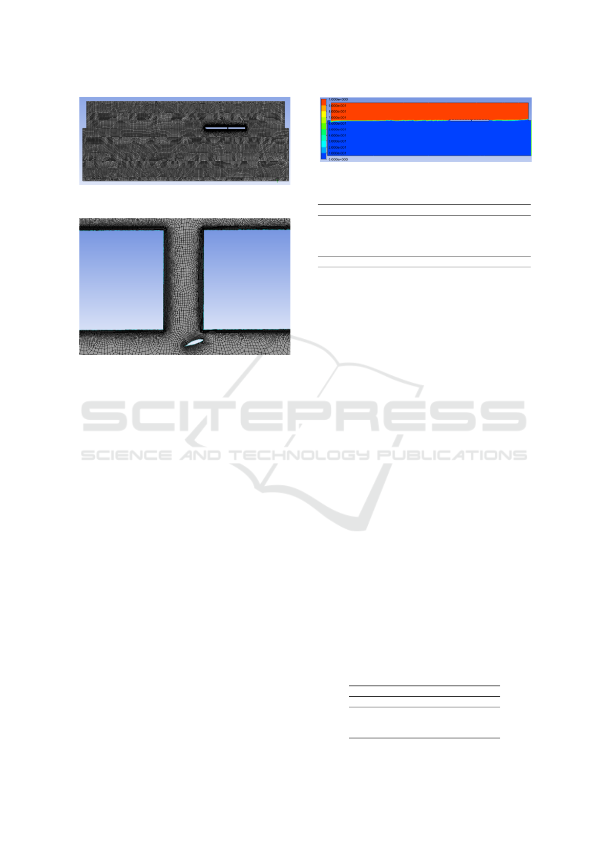
Figure 4: Mesh Model (No. of Nodes = 201775; No. of

elements = 196401)

Figure 5: Enlarged View of Mesh for Part B (clearance =

20mm, angle of attack=20

◦

)

2.3 Grid and Discretization

A sample of mesh model for the setup is shown in

Figure. 4. Quadrilateral is applied for the meshing

method as it gives more even separation for the air-

water interface of the domain. The value for the mesh

is done by trial and error to give the most appropriate

mesh model for the model. Because the mesh should

be evenly distributed around the model. Hence, edge

sizing and edge ﬁrst layer thickness inﬂation also im-

plemented in the model to give narrower and more

even grid distribution towards the surface of the 2D-

model. The volume fraction of air is given as 1 for

the segment FGIJ, and 0 for the segment EFHI. In

this work, second order upwind scheme is used in all

calculation using a pressure-based computation. All

numerical simulation is done using transient solution.

The convergence criterion for numerical parameters

are all set to 10-3 for velocity, continuity, k, and ω.The

time step used in simulation is 0.001s with number of

time steps of 20 and 20 iterations.

The volume fraction of air is given as 1 for the seg-

ment FGIJ, and 0 for the segment EFHI. In this work,

second order upwind scheme is used in all calcula-

tion using a pressure-based computation. All numer-

ical simulation is done using transient solution. The

convergence criterion for numerical parameters are all

set to 10-3 for velocity, continuity, k, and ω The time

step used in simulation is 0.001s with number of time

Figure 6: Two Dimensional Representation of Air-water In-

terface on Computational Domain

Table 2: Numerical Data

Type θ

◦

(N) ∆D

(N) %∆R Error

Bare Plate Bare 173.48 - - 4.41%

WAIP 12 155.24 -18.24 10.51 7.46%

WAIP 16 156.63 -16.86 9.72 6.08%

WAIP 20 177.53 4.05 -2.33 9.02%

Error 6.74%

steps of 20 and 20 iterations. The numerical simula-

tion of the same geometry is adopted and similar sim-

ulations were performed for the validation purposes.

Since some of vital data such as plate draught, and the

length of afterbody were not reported in the paper, the

validation is somewhat approximate and shows error

of 6.74%. From the result obtained, it is concluded

that Volume of Fluid model and k-ω SST turbulence

model are the appropriate computational model for

this case of problem.

3 RESULTS AND DISCUSSIONS

The drag on the part C is showed in Table 3, 4,

and 5 for each conﬁguration of clearance of 10 mm,

15 mm, 20 mm respectively, and angle of attack of the

hydrofoil of 12

◦

, 16

◦

, and 20

◦

, where F

, F

, C

are

pressure drag, viscous drag, total drag, and coefﬁcient

of pressure respectively.

A visualization of total drag experienced by part C

is shown in Figure. 7 for each clearance of 10 mm, 15

mm, and 20 mm respectively. The simulation is con-

ducted without performing air injection from the hull

pipe in the WAIP device to proof the critical velocity

in (1) could produce the phenomenon of air entrain-

ment due to the negative pressure produced by the hy-

drofoil. The critical velocity of 5.6 m/s is used in the

simulation according to previous experiment (Kuma-

gai et al., 2010). The result of total drag from part

Table 3: Pressure and Viscous Drag of Part C (clearance =

10 mm; Re = 1.49 x 10

)

Clearance 10 mm

◦

12 97.03 97.03 158.41 158.41

16 97.64 97.64 159.42 159.42

20 96.80 96.80 158.04 158.04

SENTA 2018 - The 3rd International Conference on Marine Technology

166

C shows the distribution of the obtained data has no

particular tendency. On the clearance of 10 mm, the

smallest value of total drag is obtained in the angle

of attack of 20

◦

which has a very small difference in

value compares to the 12

◦

, and reach the maximum

value at 16

◦

. Otherwise, on the clearance of 20 mm,

the minimum value is obtained at 16

◦

Table 4: Pressure and Viscous Drag of Part C (clearance =

20 mm; Re = 1.49 x 10

Clearance 20 mm

◦

12 105.11 105.11 171.61 171.61

16 104.37 104.37 170.40 170.40

20 105.03 105.03 171.48 171.48

Table 5: Pressure and viscous drag of part C (clearance =

15 mm; Re = 1.49 x 10

)

Clearance 15 mm

◦

12 95.09 95.09 155.24 155.24

16 95.93 95.93 156.63 156.63

20 108.74 108.74 177.53 177.53

Table 6: Pressure and Viscous Drag of Part C (clearance =

10 mm; Re = 1.49 x 10

Clearance 10 mm

◦

12 49.13 3.41 52.54 80.22 5.57 85.79

16 74.85 3.18 78.04 122.21 5.19 127.41

20 91.41 2.60 94.01 149.24 4.25 153.49

However, on the clearance of 15 mm, the mag-

nitude of total drag increased drastically. This phe-

nomenon caused by the ﬂow of the ﬂuid that occurs

due to the presence of hydrofoil. The ﬂuid ﬂow oc-

curs on the downstream side of the hydrofoil is dif-

ﬁcult to be mapped as a function. Hydrofoil always

has a tendency to experienced larger value of drag as

the angle of attack increased (Ockfen and Matveev,

2009). However, in this case study is performed to

analyze the effect produced by the hydrofoil towards

the total drag experienced on part C, the results could

not explain explicitly whether the data has a tendency

towards particular trends. A large number of varia-

tions of angle of attack is needed to really ﬁnd the

exact plot of the phenomena. In the previous work

(Kumagai et al., 2011) also said that the fundamental

ﬂow physics concerning this facility has not been clar-

iﬁed yet because extremely complicated phenomena,

which are the free-surface effect of the hydrofoil.

However, from the result above it is can be ob-

tained that the 10 mm clearance gives the smallest

value of mean total drag. The zero value of the pres-

sure drag of the part C is due to the ﬂow stream does

not cross the plate, instead the ﬂow is parallel to the

plate. Thus, the plate only experienced viscous drag

due to the viscosity of the ﬂuid. On the WAIP (part

B), the total drag is obtained by summing the pressure

drag and viscous drag experienced by the hydrofoil.

The drag component of each clearance of 10 mm, 15

mm, and 20 mm respectively is shown in Table 6, 7

and 8.

Table 7: Pressure and viscous drag of part C (clearance =

15 mm; Re = 1.49 x 10

Clearance 15 mm

◦

12 43.33 3.31 46.64 70.74 5.41 76.15

16 71.48 3.36 74.83 116.70 5.48 122.18

20 192.79 1.82 194.61 314.75 2.97 317.73

Table 8: Pressure and viscous drag of part C (clearance =

20 mm; Re = 1.49 x 10

Clearance 20 mm

◦

12 78.66 2.64 81.30 128.42 4.31 132.73

16 133.53 2.04 135.57 218.01 3.32 221.34

20 195.03 1.59 196.62 318.41 2.60 321.01

Table 9: Drag Force on Bottom Plate of The Model

Clear. θ

◦

Do Db Dt Db

- bare 174.76 173.48 348.24 -

10mm

12 85.79 158.41 244.20 -15.07

16 127.41 159.42 286.82 -14.06

20 153.49 158.04 311.54 -15.44

15mm

12 76.15 155.24 231.39 -18.24

16 122.18 156.63 278.80 -16.86

20 465.42 177.53 642.95 4.05

20mm

12 132.73 171.61 304.34 -1.88

16 221.34 170.40 391.74 -3.08

20 321.01 171.48 492.49 -2.00

The hydrofoil experienced pressure drag due to its

surface intersecting the ﬂuid’s streamline. Thus, the

molecule impacts the surface of the hydrofoil and re-

sulting non-zero value of pressure drag. The visual-

ization of the inﬂuence of clearance and angle of at-

tack on pressure coefﬁcient of the hydrofoil is shown

in Figure 8. As can be seen on Figure 8, the pres-

sure coefﬁcient of the hydrofoil has a tendency to in-

crease as the angle of attack increase. As theoretically

expected, the drag force increase as the angle of at-

tack is increased (Ockfen and Matveev, 2009). The

increased of angle of attack resulting in increase of

angle from intersection line between the hydrofoil’s

chord line and the ﬂuid’s streamline. As a result, a

larger amount of energy to deﬂect the stream is re-

quired. The energy is obtained from kinetic energy

which in this case is the moving ﬂuid. On the actual

Numerical Study on Inﬂuence of Hydrofoil Clearance towards Total Drag Reduction on Winged Air Induction Pipe for Air Lubrication

167

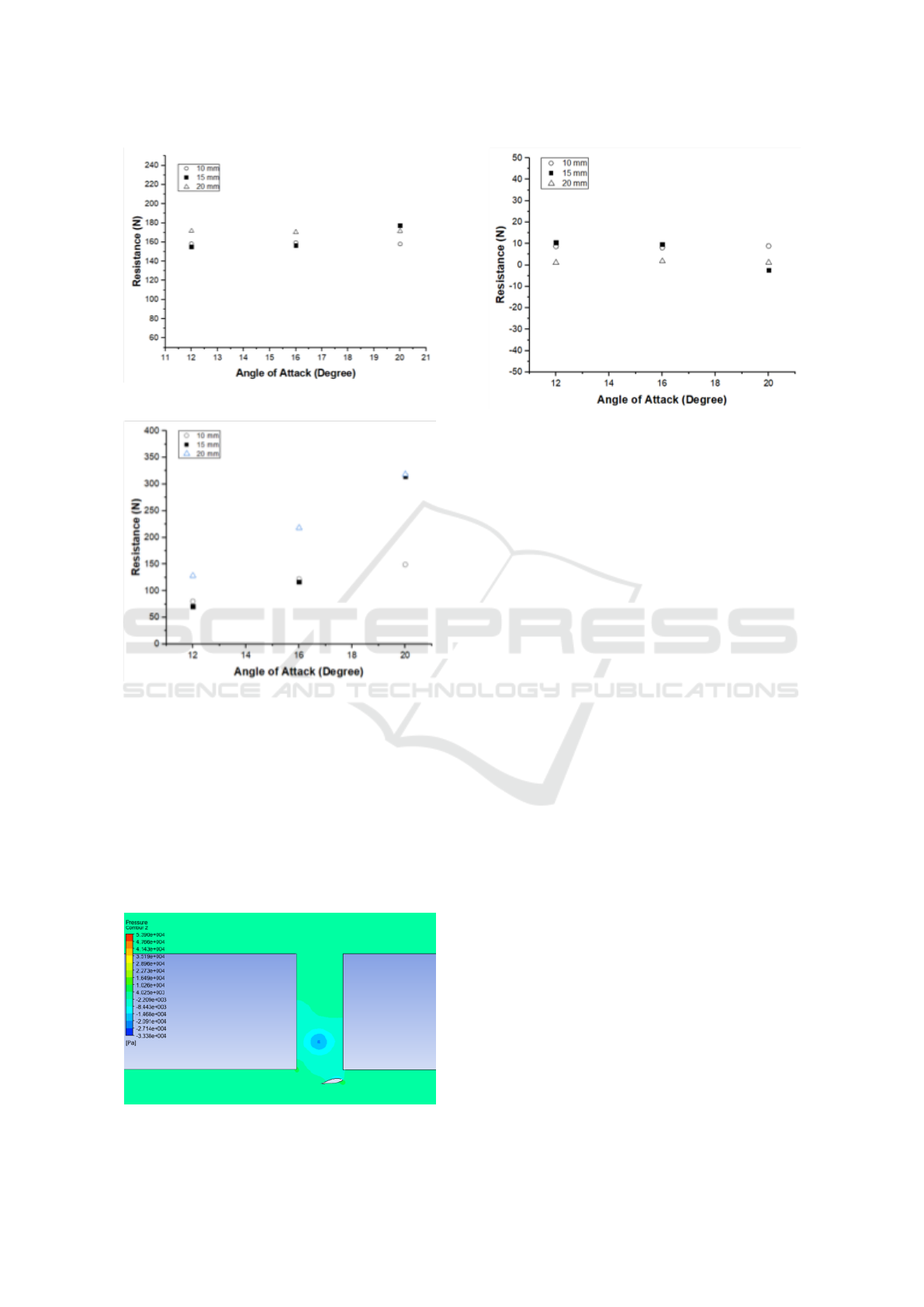
Figure 7: Total Drag Experienced by Part C

Figure 8: Pressure coefﬁcient of the hydrofoil

condition, the model is moving through the water re-

sulting the kinetic energy is produced by the object

instead of the ﬂuid. Thus, the energy loss is experi-

enced by the model. However, since the study is to

analyze the drag experienced by part C, further anal-

ysis of the hydrofoil’s drag is not performed.

A contour plot of dynamic pressure around part B

is shown in Figure. 9. As can be seen the pressure gets

Figure 9: Contour of dynamic pressure on part B

Figure 10: Drag reduction of part C

lower in the hull pipe above the hydrofoil. The phe-

nomenon is called the negative pressure, which the

pressure is lower compares to its surrounding. The

negative pressure is produced as the ﬂuid moves to-

wards the model. The hydrofoil produces lower pres-

sure on its upper surface due to higher velocity caused

by longer curvature. experienced by part C for each

conﬁguration of the model, where Do, is the hydrofoil

total drag. On the clearance of 10 mm 8-9% of drag

reduction is obtained. However, on the clearance of

15 mm, there is an added drag of 2% on angle of at-

tack of 20

◦

. In this case the data is referred as outlier

or data that is outside the trend line (Mittnik et al.,

2001). Outlier is a common data in data distribution

that is not follow the normal distribution. This can be

caused by error from numerical computation that has

been performed where the mesh element relatively, is

not evenly distributed. As a result, the computational

result has a large value of error. The distribution of

mesh is depended on the element size of the mesh.

The element size has to be adjusted to ﬁt the model

set up regarding the distance between two or more

surface/edge of the model. Generally, as the element

of the mesh get smaller the more accurate the result

gathered. However, this is could not be corresponded

that the ﬁnest possible gives the best result. Thus,

the grid independency test has to be performed in fu-

ture work. But as the error of the numerical data is

less than 10 percent the result obtained is somewhat

approximate regarding to the validation performed.

In some modelling, to reach solution’s grid indepen-

dency, numerical value in the computational domain

(the sizing parameter of mesh element) should be

much smaller than corresponding local value of the

model so that the numerical error could be minimized

(Wang and Zhai, 2012).

SENTA 2018 - The 3rd International Conference on Marine Technology

168

4 CONCLUSIONS

Computational Fluid Dynamics approach to estimate

the drag reduction by air lubrication using Winged Air

Induction Pipe (WAIP) is performed in the present

study and reasonably validated with experimental

works. By using nine conﬁgurations to achieve the

effect of hydrofoil clearance towards the drag reduc-

tion it is concluded that: the magnitude of drag reduc-

tion can be achieved when the contributing parameter

which are the angle of attack and hydrofoil clearance

chose at their optimum range. The optimum range

is achieved by modiﬁcation of the parameter using

trial and error method. The modiﬁcation of hydro-

foil clearance of the WAIP does not give a data trend

to a certain way. The application of WAIP gives result

of net drag reduction up to 10%. Figure 10 shows the

value of the drag reduction for each conﬁguration of

the model. The clearance of the hydrofoil gives a sig-

niﬁcant inﬂuence for the drag reduction. However, the

value of the drag reduction has no particular tendency

towards certain point. Therefore, the appropriate de-

sign is obtained by using trial and error method. This

is due to the unique ﬂow characteristic produce by the

hydrofoil interacts with the plate in part C in different

ways depend on the clearance between hydrofoil

ACKNOWLEDGEMENTS

Authors are thanks to Department of Mechanical En-

gineering, Faculty of Engineering, Universitas In-

donesia for making facility available and also grant

PITTA No. 2561/UN2.R3.1/HKP05.00/2018

REFERENCES

Cui, Z., Fan, J. M., and Park, A. H. (2003). Drag coefﬁ-

cients for a settling sphere with microbubble drag reduc-

tion effects. Powder Technology, pages 132–134.

Duncan, J. H. (1981). An Experimental Investigation of

Breaking Waves Produced by a Towed Hydrofoil. Pro-

ceedings of the Royal Society of London. Series A, Math-

ematical and Physical Sciences, 377(1770):331–348.

Evans, G. M., Jameson, G. J., and Atkinson, B. W. (1992).

Prediction of the bubble size generated by a plunging liq-

uid jet bubble column. Chemical Engineering Science,

47:3265–3272.

Kodama, Y., Kakugawa, A., Takahashi, T., and Kawashima,

H. (2000). Experimental study on microbubbles and their

applicability to ships for skin friction reduction. In In-

ternational Journal of Heat and Fluid Flow, pages 582–

588.

Kumagai, I., Kushida, T., Oyabu, K., Tasaka, Y., and Murai,

Y. (2011). FLOW BEHAVIOR AROUND A HYDRO-

FOIL CLOSE TO A FREE SURFACE. Vis Mech Proc

Visualization of Mechanical Processes, 1(4).

Kumagai, I., Nakamura, N., Murai, Y., Tasaka, Y., Takeda,

Y., and Takahashi, Y. (2010). A New Power-saving De-

vice for Air Bubble Generation: Hydrofoil Air Pump for

Ship Drag Reduction. Proceedings of International Con-

ference on Ship Drag Reduction (SMOOTH-SHIPS).

Kumagai, I., Takahashi, Y., and Murai, Y. (2015). Power-

saving device for air bubble generation using a hydrofoil

to reduce ship drag: Theory, experiments, and applica-

tion to ships. Ocean Engineering, 95:183–195.

Menter, F. R. (1994). Two-equation eddy-viscosity turbu-

lence models for engineering applications. AIAA Jour-

nal, 32:1598–1605.

Mittnik, S., Rachev, S. T., and Samorodnitsky, G. (2001).

The distribution of test statistics for outlier detection

in heavy-tailed samples. Mathematical and Computer

Modelling, 34:1171–1183.

Mohanarangam, K., Cheung, S. C., Tu, J. Y., and Chen,

L. (2009). Numerical simulation of micro-bubble drag

reduction using population balance model. Ocean Engi-

neering, 36:863–872.

Muratoglu, A. and Yuce, M. I. (2015). Performance Anal-

ysis of Hydrokinetic Turbine Blade Sections. Technical

report.

Muste, M., Yu, K., Fujita, I., and Ettema, R. (2009). Two-

phase ﬂow insights into open-channel ﬂows with sus-

pended particles of different densities. Environmental

Fluid Mechanics, pages 161–186.

Ockfen, A. E. and Matveev, K. I. (2009). Aerodynamic

characteristics of NACA 4412 airfoil section with ﬂap in

extreme ground effect. International Journal of Naval

Architecture and Ocean Engineering, 1:1–12.

Pang, M. J., Wei, J. J., and Yu, B. (2014). Numerical study

on modulation of microbubbles on turbulence frictional

drag in a horizontal channel. Ocean Engineering, 81:58–

68.

Shereena, S. G., Vengadesan, S., Idichandyxs, V. G., and

Bhattacharyya, S. K. (2013). CFD study of drag reduc-

tion in axisymmetric underwater vehicles using air jets.

Engineering Applications of Computational Fluid Me-

chanics, 7:193–209.

Toffoli, A., Babanin, A., Onorato, M., and Waseda, T.

(2010). Maximum steepness of oceanic waves: ﬁeld

and laboratory experiments. Geophysics Research Let-

ters, 37.

Wang, H. and Zhai, Z. J. (2012). Analyzing grid indepen-

dency and numerical viscosity of computational ﬂuid dy-

namics for indoor environment applications. Building

and Environment, 52:107–118.

Yanuar, Gunawan, Sunaryo, and Jamaluddin, A. (2012).

Micro-bubble drag reduction on a high speed vessel

model. Journal of Marine Science and Application,

11:301–304.

Numerical Study on Inﬂuence of Hydrofoil Clearance towards Total Drag Reduction on Winged Air Induction Pipe for Air Lubrication

169

REFERENCES

Cui, Z., Fan, J. M., and Park, A. H. (2003). Drag coeffi-