
Developing the Developable Surfaces in a Space to the Plane using
Some Triangle Pieces
Kusno and Nur Hardiani
Jember University, Jl. Kalimantan No. 37, Jember, Indonesia
Department of Tadris Matematika, State Islam University, Mataram, Indonesia
Keywords: Developing, Developable Surfaces, Space, Plane, Triangle.
Abstract: This paper deals with the development in the space to the plane of the polygons, the cone, the cylindrical
surfaces and the developable quartic Bézier patches in which its boundary curves are respectively parallel,
and the normal vectors of the surfaces must be in the same orientation. The method is as follows, we
approximate the surfaces into some triangle pieces then we transform consecutively these pieces in the plane.
The result of the study shows that the use of the triangle approximation method can develop effectively these
surfaces in the space to the plane. In addition, it can be applied to detect all surface measures of an object that
are defined by those surface types.
1 INTRODUCTION
Some methods related to the development of surface
to the plane have been presented. The development of
the pipeline surfaces can be carried out by
enumerating of two boundary curves in some
approximation polygons (Weiss and Furtner, 1998).
We can develop a surface to the plane by using the
techniques of interactive piecewise flattening of
parametric 3-D surfaces, leading to a non-distorted
(Bennis and Gagalowicz, 1991). After that,
developing an arbitrary developable surface into a
flattened pattern is based on the geodesic curve length
preservation and linear mapping principles
(Clements, 1991; Gan et al., 1996). We can simulate
the physical model of transitional pipeline parts
whose cross sections are plane curve and polygon and
are made of unwrinkled or unstretched materials. It is
based on the approximation of the boundary surface
triangulation (Obradović et al., 2014). Different from
the previous methods, we are interested in the
discussion about the development of the convex
polygons, the conic/cylindrical surfaces and the
developable quartic Bezier patches in a space to the
plane using the triangle pieces.
This paper is organized in the following steps. In
the first, we talk about the development of the triangle
and polygon plane surfaces in space to the plane. In
the second, we evaluate the development of the cone
and the cylinder defined by the linear interpolation of
two parallel circles. In the third, the construction and
the development of developable quartic Bezier
patches in a space to the plane are introduced. Finally,
the results will be summarized in the conclusion
section.
2 DEVELOPING THE TRIANGLE
AND THE POLYGON PLANE
SURFACE IN A SPACE TO THE
PLANE
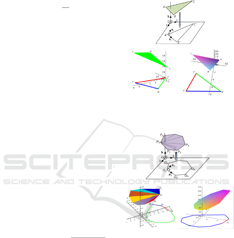
Let a triangle plane . The vector
and
form an angle in the space orthonormal coordinate
. The problem is how to develop the plane
in the plane orthonormal coordinate in
which the vector
of the side development of
triangle is align to the determined unit vector
(Figure 1a).
To develop the triangle in space to the
plane can be undertaken as follows (Gan et
al., 1996).
1). Determine the vector′′
and
calculate the unit vector
.
2). Evaluate the measure of angle
Kusno, . and Hardiani, N.
Developing the Developable Surfaces in a Space to the Plane using Some Triangle Pieces.
DOI: 10.5220/0008523104270431
In Proceedings of the International Conference on Mathematics and Islam (ICMIs 2018), pages 427-431
ISBN: 978-989-758-407-7
Copyright
c
2020 by SCITEPRESS – Science and Technology Publications, Lda. All rights reserved
427
.
3). Calculate
4). Construct the developed triangle in the
plane orthonormal coordinate by using
the linear interpolation of the couple points ,
and that are
(1)
with .
If the positions and are ,
and , then we will find the
development of the triangle as it is shown in Figure
1b. If the positions , and are ,
and , its development is shown in
Figure 1(c).
Consider a piece of convex polygon plane Ꝑ of
the vertices
in space that are
shown in Figure 2a. The development of the polygon
to the plane orthonormal coordinate can be
carried out as follows.
1). Determine an initial point of the development
and two orthonormal unit vectors
.
2). Determine a point
that is an image of the point
such that
.
3). Calculate the length
for
and evaluate the measure of the angle
for .
4). Evaluate the points
for in the
plane as the images
by
using the formula
.
5). Using equation (1), construct the polygon of
development
in the plane .
(a)
(b)
(c)
Figure 1: (a) Calculation of the angle
in the plane
, (b) Development of triangle plane in space to
the plane by starting point at , and (c) by
starting point at .
(a)
(b)
(c)
Figure 2: (a) Calculation of the angles
for
of the convex polygon
in the plane
, (b) Decomposition of the polygon
into
some triangles, (c) Development of the convex polygon
to the plane .
In case of the polygon vertices P
1
(0,-0,7), P
2
(4,-
12,7), P
3
(8,-5,7), P
4
(9,0,7), P
5
(5,3,7), P
6
(0,4,7), P
7
(-
3,3,7), P
8
(-4,0,7) and P
9
(-3,-5,7) that are lied in the
plane z =7, the development of the polygon in plane
can be shown in Figure 2b. If the polygon vertices
P
1
(0,-10,18), P
2
(4,-12,16), P
3
(8,-5, 5), P
4
(7,0,1),
P
5
(4,3,1), P
6
(0,4,4), P
7
(-3,3,8), P
8
(-4,0,12) and P
9
(-
3,-5,16) are determined in the planex + y + z - 8= 0,
then the result of development is shown in Figure 2c.
ICMIs 2018 - International Conference on Mathematics and Islam
428
In the more general cases, if we are given a series
of consecutive triangles plane in space [P
1
P
2
P
3
,
P
2
P
3
P
4
, ... , P
n
P
(n+1)
P
(n+2)
] that are defined by n+2
points P
1
, P
2
, P
3
, ..., P
(n+2)
, then the development of
the triangles to the plane can be realized
respectively by equation (1). To justify the method,
when we give the points data of triangle pieces in
space P
1
(3,0,3), P
2
(0,0,4), P
3
(3,3,2), P
4
(0,4,4),
P
5
(1,8,5) and P
6
(1,9,5), we will find its development
in the plane that are shown in Figure 3a. If the triangle
pieces are defined by the points P
1
(6,0,3), P
2
(0,1,2),
P
3
(3,3,3), P
4
(0,4,2), P
5
(1,8,3), P
6
(1,11,5), P
7
(5,8,4),
P
8
(1,12,4), P
9
(10,12,3) and P
10
(7,14,4), then its
development in the plane are shown in Figure 3b.
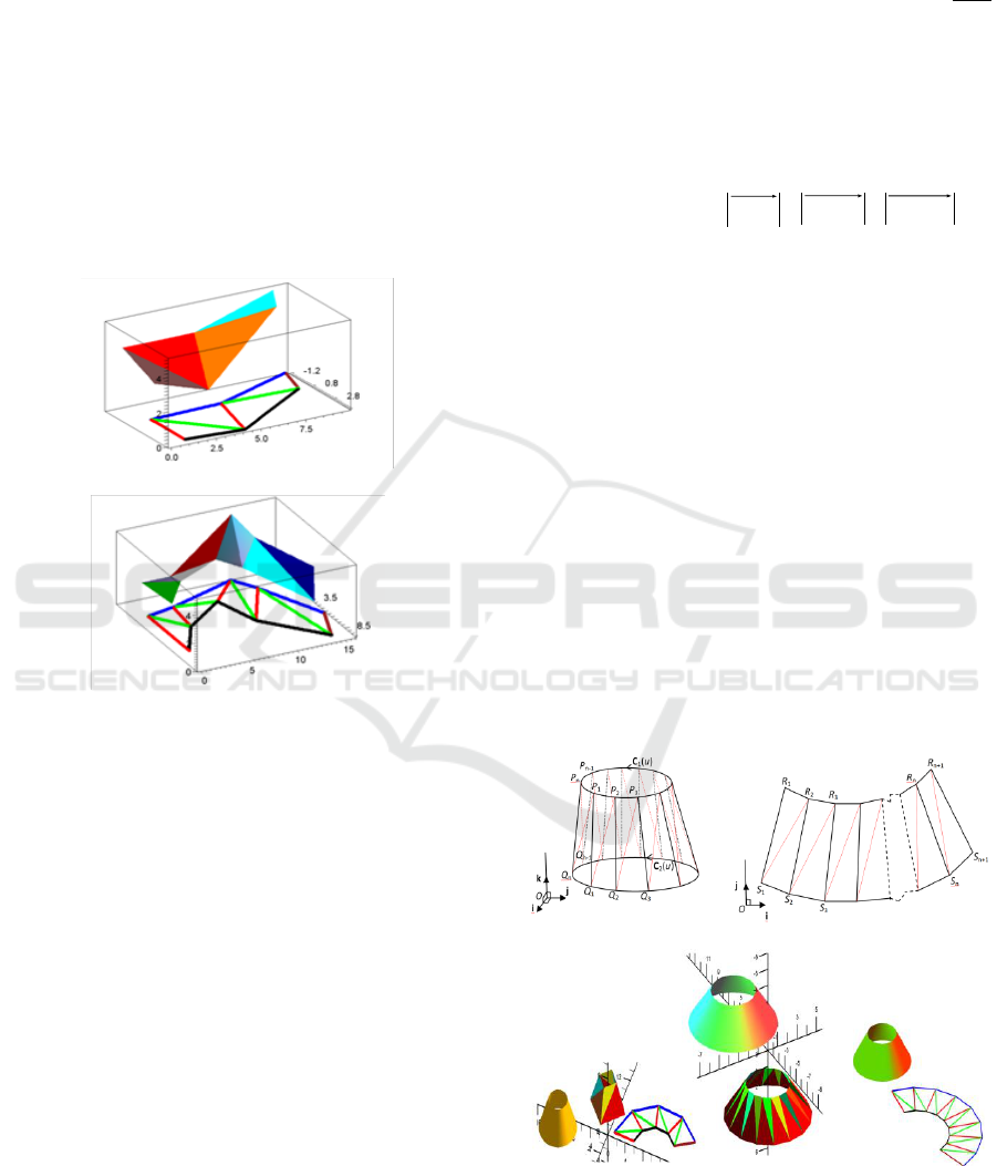
(a)
(b)
Figure 3: (a) Development of four triangles plane series
toplane, (b) Development of eight triangles plane series to
plane.
3 DEVELOPING THE CONE AND
THE CYLINDER OF TWO
CIRCLES LINEAR
INTERPOLATION
Consider a cone or a cylinder surfaces S(u,v) = (1-v)
C
1
(u) + vC
2
(u) in which its boundary curves C
1
(u)
and C
2
(u) are the parallel circles
C
1
(u) = < r
1
cos u + a, r
1
sin u + b, z
C1
> (2)
and
C
2
(u) = < r
2
cos u + c, r
2
sin u +d, z
C2
>
with radius r
1
, r
2
and the value a, b, z
C1
, c, d, z
C2
real
constants, 0 u 2 and 0 v 1. Developing the
surface S(u,v) to the plane [O,i,j] can be carried out
by using the triangles approximation as follows
(Figure 4a,b).
1) Determine the (n +1) parameter values u
i
=
(2) of i = 1, 2, 3, ..., (n+1) to define the 2n
triangle plane pieces [P
1
Q
1
P
2
, P
2
Q
1
Q
2
, P
2
Q
2
P
3
,
..., P
n
Q
n
P
n+1
, P
n+1
Q
n
Q
n+1
]. The point P
i
is
defined by C
1
(u
i
) and the point Q
i
is defined by
C
2
(u
i
) for i = 1, 2, 3, ..., n+1 with P
n+1
= P
1
and
Q
i+1
= Q
1
.
2) Calculate the length
ii
PQ
,
1ii
PQ
,
1ii
QQ
and
the measure of consecutive angles
1
iii
PQP
and
11
iii
QQP
for i = 1, 2, 3, ..., n.
3) In the plane [O,i,j], determine an initial point
of development S
1
and two orthonormal vectors
a
1
a
2
. Using the triangle development method in
section 2 and the determined initial point S
1
can
be developed respectively and consecutively the
triangles [P
1
Q
1
P
2
, P
2
Q
1
Q
2
, P
2
Q
2
P
3
,..., P
n
Q
n
P
n+1
,
P
n+1
Q
n
Q
n+1
] in space to the plane [O,i,j] that are
[R
1
S
1
R
2
, R
2
S
1
S
2
, R
2
S
2
R
3
, ..., R
n
S
n
R
n+1
,
R
(n+1)
S
n
S
(n+1)
].
If C
1
(u) = <2cos u + 1, 2 sin u - 3, 4> and C
2
(u) =
<4cos u + 1, 4 sin u - 3, 2>, then the development of
the conic surface S(u,v) into 8 triangles to the plane
[O,i,j] is shown in Figure 4c. In the Figure 4d, we
present a cone approximated by 32 triangles. The
Figure 4e show the development of the conic surface
into 16 triangles to the plane [O,i,j].
(a) (b)
(c)
Figure 4: (a) Decomposition a cone into some triangles, (b)
Development of the cone to the plane [O,i,j], (c)
Development examples of the pyramid and the cone to
plane.
Developing the Developable Surfaces in a Space to the Plane using Some Triangle Pieces
429

4
DEVELOPING THE DEVELOPABLE
QUARTIC BEZIER PATCHES IN
A SPACE TO THE PLANE
The developable surfaces are local properties of the
surface. It is not only in the form of the plane surface
but also in the form of the conic, the cylindrical and
the tangent lines surfaces (Lipschultz, 1969; Kusno,
1998). This section discusses about the definition of
developable quartic Bézier patches supported by two
parallel plane and then talk about the developing of
the patches in the plane using the method of the
triangle approximation. We analyze as follows.
Let the quartic Bézier curves
C
1
(u) and
C
2
(u)
in the form
, (3)
and
,
with
and 0 ≤ u ≤ 1.
Because of the application reason, the curves
C
1
(u) and C
2
(u) are lied respectively in two parallel
planes [Ψ
1
,Ψ
2
]. So, by using the developable
condition of regular developable surfaces, it must be
formulated in the form (Frey and Bindschadler, 1993;
Kusno, 1998)
C
′
2
(u) = ρ(u) C
′
1
(u), (4)
with the real scalar ρ(u)> 0. In order to simplify the
calculation, we choose the scalar ρ(u) positive
constant i.e. ρ(u) = α
R
+
. From the condition (4), we
will find
(5)
The polynomials
are not zero for i = 0, 1, 2, 3
thus
[(q
i
−q
i+1
) + α.(p
i+1
−p
i
)] = 0, (6)
for all . When we add those equations,
we will find an equation of the Bézier polygon
control points of the curves C
1
(u) and C
2
(u) as
follows
[(q
4
−q
0
) = α.(p
4
−p
0
)]. (7)
So, to construct a regular developable Bézier
patch which is supported by two curves C
1
(u) and
C
2
(u) of degree 4 and conditioned by ρ(u) positive
constant must be verify the equation (4) and (5),
namely
1. the two vectors parallel (q
4
−q
0
) and (p
4
−p
0
) must
be in the same direction to calculate α value such
that
(8)
2. every the vector (q
i+1
−q
i
) and
(p
i+1
−p
i
) must be parallel and proportional to α.
Furthermore, to facilitate the continuous connection
of two adjacent patches, in equation (4), must be
necessary to determine four boundary control points
[p
o
,q
o
,p
4
,q
4
] of the Bézier curve C
1
(u), C
2
(u) and
two control points [p
1
,p
3
] of the Bézier curve C
1
(u).
Therefore, if we determine the control points
[p
0
,p
1
,p
3
,p
4
,q
0
,q
4
], then from the equations (4) we
will find respectively four equations to calculate the
control points [q
1
,q
3
,q
2
,p
2
] in the form
q
1
= q
0
+ α.(p
1
− p
0
); q
3
= q
4
− α.(p
4
− p
3
); (9)
q
2
= ½ (q
1
+ q
3
); p
2
= ½ (p
1
+ p
3
).
Thus, using the data control points [p
0
,p
1
,p
3
,p
4
,q
0
,q
4
],
equation system (6) and equation (8) can determine
the control points [q
1
,q
2
,q
3
,p
2
]. All these control
points can define the developable quartic Bézier patch
of equation (4). In addition, if we fix in equation (8)
the value α = 1 and α > 1, then we will find
respectively the developable cylindrical patches and
the developable conic patches.
(a)
(b)
Figure 5: (a) Two examples of the
developable quartic
Bézier patches, (b) development of the developable quartic
Bézier patch in a space to plane by using some triangles.
ICMIs 2018 - International Conference on Mathematics and Islam
430

To justify this method and develop its result surface
in a space to the plane, we simulate as follows. If we
substitute in equation system (6) the control points
data p
0
,=<35,-95,0>, p
1
=<35,-60,65>, p
3
=<35,0,-
45>,p
4
= <35,95,0>,q
0
=<-40,-100,25> andq
4
=<-
40,116,25>, then the solution will find the control
points q
1
=<-40,-51,116>, q
2
= <-40,-9,39>,q
3
=<-
40,33,-38>,p
2
=<35,-30,10> that are define the
developable quartic Bézier patch in Figure 5a,b.
Furthermore, the Figure 5c,d represent the
development of the developable quartic Bézier
patch to the plane using the triangles approximation
method.
5 CONCLUSIONS
By using the triangles approximation method, we
presented the development in the plane of some
developable surfaces in which its boundary curves are
respectively parallel, and the normal vectors of the
surface must be in the same orientation. It is very
useful to develop the polygon plane, the conic, the
cylindrical surfaces or
the
developable quartic Bézier
patches. Therefore, it can be applied to detect all
surface measures of an object that are defined by
those surface types.
The development of the polygon plane, the conic,
the cylindrical surfaces or
the
developable quartic
Bézier patches have been introduced. The interesting
thing to discuss ahead is how to define and develop in
plane
the
developable Bézier patches of high degrees.
REFERENCES
Bennis, C., Gagalowicz, A., 1991. Piecewise Surface
Ftattening for Non-Distorted Texture Mapping.
Computer Graphics, vol. 25, pp. 237-246.
Clements, J. A., 1981. Computer System to Derive
Developable Hull Surface and Tables of Offsets.
Marine Technology, vol. 8, pp. 221-233.
Frey W. H., Bindschadler, D., 1993. Computer-Aided
Design of a Class of Developable Bézier Surfaces
(USA: R and D Publication 8057, General Motors).
Gan, M. C., Tan S. T. &Chan, K. W., 1996. Flattening
Developable Bi-parametric Surfaces. Computers &
Structures, vol. 58, pp.703-708.
Kusno, 1998. Contribution a la Solution du Problėm de
Construction et de Raccordement Géométrique de
Surfaces Développables Réguliėrs a l'Aides de
Carreaux de Bézier, Thėse de Docteur-Université de
Metz, France.
Kusno, 2010. Geometri Rancang Bangun. Jember
University Press.
Lipschultz, M.1969. Theory and Problems of Di
erential
Geometry. Schaum's Outline Series McGraw-Hill New
York.
Obradović, R., Beljin B. & Popkonstantinović B., 2014.
Approximation of Transitional Developable Surfaces
between Plane Curve and Polygon. Acta Polytechnica
Hungarica, vol. 11, pp. 217-238.
Weiss G., Furtner, P., 1988. Computer-Aided Treatment of
Developable Surfaces. Computer & Graphics, vol. 12,
pp. 39-51.
Developing the Developable Surfaces in a Space to the Plane using Some Triangle Pieces
431
