
Regression for Trend-Seasonal Longitudinal Data Pattern:
Linear and Fourier Series Estimator
M. Fariz Fadillah Mardianto
1
, Sri Haryatmi Kartiko
2
and Herni Utami
3
1
Department of Mathematics, University of Airlangga, Surabaya, Indonesia
1
Ph.D. Candidate in Department of Mathematics, University of Gadjah Mada, Yogyakarta, Indonesia
2,3
Department of Mathematics, University of Gadjah Mada, Yogyakarta, Indonesia
Keywords: Longitudinal Data, Trend Seasonal Pattern, Regression, Linear Estimator, Fourier Series Estimator.
Abstract: Longitudinal data is a pattern that consists of time series and cross section data pattern. In a research with
longitudinal and panel data often be used combination between trend and seasonal or trend-seasonal pattern,
for example the relationship between profit and demand for seasonal commodities, in education insurance,
meteorology case and many more for many subjects. Recently, we develop Fourier series estimator to
approach curve regression for longitudinal data. Fourier series that be used, not only include trigonometric
Fourier series which usual be used in Mathematics, but also linear function. In this research we compare
performance of new estimator with linear estimator that often be used in panel data regression or parametric
regression for longitudinal data. The trend-seasonal data that be used in this analysis is gotten from
simulation process based on Box et.al., (1976). The Fourier series estimator gives better result with
goodness indicator smaller Mean Square Error (MSE) and greater determination coefficient than linear
estimator.
1 INTRODUCTION
Recently, longitudinal data analysis develops for
some Statistical method. Longitudinal data is a
pattern that consists of more than one subject. Each
subject is observed more than one time. Therefore,
in longitudinal data structure, consist of time series
and cross section data pattern (Weiss, 2005).
In regression analysis, one of statistical method
that be used to model the relationship between
responses and predictors, longitudinal data analysis
often be used. Panel data regression is one of the
linear regressions for longitudinal data. The
differences between longitudinal and panel data,
panel data is longitudinal data with the number of
observations and periods are same for every subject
(Baltagi, 2005).
Regression analysis that be developed is not only
regression with linear estimator, but also
nonparametric regression. Nonparametric regression
is a Statistical modeling that be used to overcome
the relationship between responses and predictors
which have unknown pattern. Nonparametric
regression is an alternative method that be used
when the result of regression analysis with certain
function, such as linear regression, cannot suitable
with goodness criteria of regression analysis
(Takezawa, 2006). The advantage of nonparametric
regression is having high flexibility. Flexibility
means that the pattern of data that presented on the
scatter plot can determine the shape of regression
curve based on estimators in the nonparametric
regression (Budiantara et.al., 2015). Based on plot,
we can identify the pattern of data, the pattern of
pairs data, a response versus a predictor variable
data, have trend, oscillation, uncertain pattern, and
combination pattern.
The pattern of data that often be found is
combination between trend and seasonal or trend-
seasonal data pattern. In research with longitudinal
and panel data this pattern often be encountered.
Some example like, the relationship between profit
and demand for seasonal commodities, in education
insurance, meteorology case and many more for
many subjects.
Trend – seasonal data pattern popular in time
series data analysis. This pattern will pass some
procedure when time series analysis be used, be-
because there are some assumptions must be
satisfied. Time series – regression approach is an
350
M. Fariz Fadillah Mardianto, ., Kartiko, S. and Utami, H.
Regression for Trend-Seasonal Longitudinal Data Pattern: Linear and Fourier Series Estimator.
DOI: 10.5220/0008521803500356
In Proceedings of the International Conference on Mathematics and Islam (ICMIs 2018), pages 350-356
ISBN: 978-989-758-407-7
Copyright
c
2020 by SCITEPRESS – Science and Technology Publications, Lda. All rights reserved

alternative to forecast time series data (Bloomfield,
2000). Based on that concept, trend – seasonal data
pattern analysis is applied to longitudinal data, that
consist of time series and cross section data pattern.
Regression for longitudinal data pattern that be
discussed in this study based on linear and Fourier
series estimator. Linear estimator represents trend
pattern, and Fourier series represents seasonal
pattern. Bilodeau (1992) proposed combination
linear function and Fourier cosine series in his paper
to get smooth estimator for the relationship of a
response and predictors. In longitudinal analysis,
linear estimator often be used, especially in
regression, the most popular method is panel data
regression. However, that method is not suitable
when the variation of oscillation is large. So, we
propose new method based on the development of
Bilodeau (1992). The method is longitudinal data
regression based on Fourier series estimator that
consist of linear function, cosine and sine function.
Visually and mathematically, that estimator
accommodates trend-seasonal pattern that be
presented in scatter plot and time series plot for
longitudinal data.
In this paper, second part discuss about linear
estimator for longitudinal data regression. The third
part discuss about Fourier series estimator for
longitudinal data regression. Fourier series that be
used based on Fourier series estimator that consist of
linear function, cosine and sine function. Using
simulation data, we make comparison based on MSE
and determination coefficient value to make
conclusion which regression method that suitable to
be used for trend – seasonal longitudinal data
pattern. In the end of this part, given longitudinal
data structure in Table 1 as follows:
Table 1: The structure of longitudinal data that be used.
Subject
Response
Predictors
1
st
Subject
2
nd
Subject
n
th
Subject
2 LINEAR ESTIMATORS FOR
LONGITUDINAL DATA
REGRESSION
Linear estimator for longitudinal data regression is
analogue with common effect model in panel data
regression. Gujarati (2004) stated that general
approach that have similarity with generalized linear
model in panel data case is common effect model.
Consider pair of predictor and response
data
, with represents the
number of subjects,
represents the
number of observations for each subject, and
represents the number of predictors. The
structure of data pair has presented on Table 1.
Based on pair of data can be formed regression
model for longitudinal data based on linear approach
as follows:
(1)
with
is an intercept parameter for
subject,
is
parameter for
predictor and
subject. Random
error for
subject and
observation denoted by
that independent and identically normal
distributed with mean equals to 0 and variance
equals to
. An estimator for parameter which be
formed as vector for equation (1) can be determined
based on Weighted Least Square (WLS)
optimization (Weiss, 2005). The WLS optimization
result given as follows:
(2)
In this case
, that have
or with vector components that
correspond are
that have
.
is a matrix that has or
, and parameter vector defined by
Regression for Trend-Seasonal Longitudinal Data Pattern: Linear and Fourier Series Estimator
351

that has . In
addition, there is
as a weight matrix with
structure as follows:
,
where
,
with variance matrix
where . The
estimator for curve regression can be determined as
follows:
(3)
In regression for longitudinal data based on
linear estimator, inference Statistics for significant
test has been provided. There are unit root test using
Augmented Dickey Fuller (ADF), simultaneous and
partial significance test (Baltagi, 2005),
heteroscedasticity test for error using Lagrange
Multiplier (Greene, 2012) and normality test using
Jarque Bera test (Baltagi, 2005). The good estimator
is estimator with small MSE value, and big
determination coefficient value.
3. FOURIER SERIES ESTIMATOR
FOR LONGITUDINAL DATA
REGRESSION
Consider a longitudinal data structure that be
presented in Table 1. Based on Table 1, there are
pairs of data with form (
,
denotes
predictor variable for
observation in
subject.
Here, denote the number of subjects,
denote the number of observations for
each subject, and represents the
number of predictors. Response variable for
observation in
subject is denoted by
. The
pairs of data that be presented in Table 1, follows
nonparametric regression equation for longitudinal
data as follows:
, (4)
represents a regression curve.
Random error for
observation in
subject is
denoted by
that independent, identically normal
distributed with mean 0, and variance
. In this
case,
approached by Fourier series as
follows:
(5)
Equation (5) is substituted to equation (4), the result
is a nonparametric regression equation for
longitudinal data that be approached by Fourier
series. Based on equation 5,
is a component
that accommodates trend pattern,
denotes
parameter that be estimated for
predictor and
subject. The other component accommodates
seasonal pattern,
is an intercept parameter for
predictor and
subject,
is the parameter of
cosine basis for
predictor,
subject, and
oscillation parameter that be inputted,
is the parameter of sine basis for
predictor,
subject, and oscillation parameter
that be inputted.
An estimator for parameter which be formed as
vector for nonparametric regression equation with
longitudinal data that be approached by Fourier
series can be determined based on Weighted Least
Square (WLS) optimization. The WLS optimization
result given as follows:
The structure of vector is same with linear
estimator for longitudinal data regression in second
part. The matrix structure of
is given as
follows:
where
equals as follows:
.
Vectors that include regression parameters denoted
by
, where
ICMIs 2018 - International Conference on Mathematics and Islam
352

In addition, there is
as a weight matrix. In
this study, two kinds of weight are used based on
Wu and Zhang (2006). There are uniform, and
variance weighted. The structure of based on
uniform weight denoted as follows:
, (6)
where denotes the total of the observations
number for all subjects. An identity matrix for
subject is denoted by
. The structure of based on
uniform weight denoted as follows:
, (7)
with variance matrix
where . The
estimator for curve regression can be determined as
follows:
, (8)
with
.(9)
In regression for longitudinal data based on
Fourier series estimator, the good estimator is
estimator with optimal oscillation parameter, small
MSE value, and big determination coefficient value.
An optimal parameter oscillation can be determined
based on the smallest Generalized Cross Validation
(GCV) value that given as follows:
, (10)
where
and hat matrix is defined with
(Tripena and
Budiantara, 2006).
4 DISCUSSIONS
In this part we concentrate to application of either
linear or Fourier series estimator for longitudinal
data regression. There are four sub sections in this
part. The first sub section we discuss about the
simulation data. The second sub section we discuss
about application for linear estimator. The third sub
section we discuss about application for Fourier
series estimator. The last sub section we compare the
goodness of estimator result based on linear and
Fourier series estimator for longitudinal data.
4.1 About the Data
Consider simulation data that consist of one
response and two predictors. The response data used
represent monthly wind velocity data in 10 cities,
whereas the predictor data used represents the
monthly average temperature in 10 cities, and the
observation period. In this case study there are 10
cities each observed for 12 months. Based on the
scatter plot between response and predictors, there
are trend – seasonal pattern.
Simulation processes have been constructed
based on the characteristics from equation (5) where
the function included of linear and trigonometric
parts. For this simulation, we concern to modified
data based on Box et al. (1976) with take
parameters. Two parameters represent trend
components and parameters represent seasonal
components that be related to trigonometric
function. This simulation based on an analogue from
the data that be presented on Box et al. (1976).
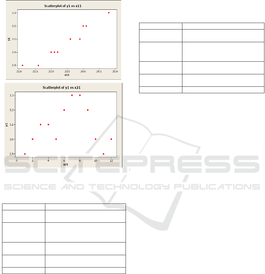
Figure 1 presents plot of data sample only for first
subject.
Based on Figure 1 it shows that there is a clear
trend pattern between the first predictor variable
with the response variable, and a clear seasonal
pattern between the second predictor variable and
the response variable. The pattern is same for the
other subject.
4.2 Linear Estimator Result
Based on simulation data, first we use two predictor
variables to estimate a response variable. The result
of the first linear regression estimation for
longitudinal data is as follows:
.
Regression for Trend-Seasonal Longitudinal Data Pattern: Linear and Fourier Series Estimator
353
The summary from the series of hypothesis test for
the first estimation is presented in Table 2.
Figure 1: Plot of data sample for first subject.
Table 2: The summary from the series of hypothesis test
for the first estimation.
Test
Result
Augmented
Dickey Fuller
Time series component stationer
Simultaneous
Parameter that be estimated affect
to response variable
simultaneously.
Partial
For second predictor (observation
period) does not significant
Lagrange
Multiplier
Heteroscedasticity is happened.
Jarque Bera
Error distribution is normal
Because of second predictor, observation period,
does not significant based on hypothesis test, so we
eliminate that predictor, and we use a predictor
variable, the first predictor, to estimate a response
variable. The result of the second linear regression
estimation for longitudinal data is as follows:
The summary from the series of hypothesis test for
the second estimation is presented in Table 3 as
follows:
Table 3: The summary from the series of hypothesis test
for the second estimation.
Test
Result
Augmented
Dickey Fuller
Time series component stationer
Simultaneous
Parameter that be estimated affect
to response variable
simultaneously.
Partial
Partially, predictor significant
based on hypothesis test.
Lagrange
Multiplier
Heteroscedasticity is happened.
JarqueBera
Error distribution is normal
The second regression model has a
determination coefficient value equals to 0.87241,
which means that the predictor can explain the
response of 87.241%. The MSE value equals to
0.1106. The determination coefficient value is big,
and the MSE value is small, so it can satisfy the
indicator of goodness estimator. However, the
weakness of the linear estimator for longitudinal
data regression in this study, the wind speed
estimation does not involve period variable, and
there are cases of heteroscedasticity in the error. The
resulting MSE value can be smaller, and the
resulting determination coefficient value can be
greater if using other approaches such as
nonparametric regression for longitudinal data.
4.3 Fourier Series Estimator Result
Furthermore, using the same data, applied to
nonparametric regression for longitudinal data based
on Fourier series estimator. The weighting types that
be used are uniform weighting and variance based
on Wu and Zhang (2006). The criterion of goodness
that be used is the small MSE value, and the large of
determination coefficient value. The optimal
oscillation parameter is determined based on
minimum GCV value. The Fourier series estimator
for nonparametric regression of longitudinal data is
determined based on equation (8). The GCV value is
calculated based on equation (10). The GCV values
based on uniform weighting for each oscillation
parameter are presented in Table 4. The GCV values
based on uniform weighting for each oscillation
parameter are presented in Table 5.
ICMIs 2018 - International Conference on Mathematics and Islam
354
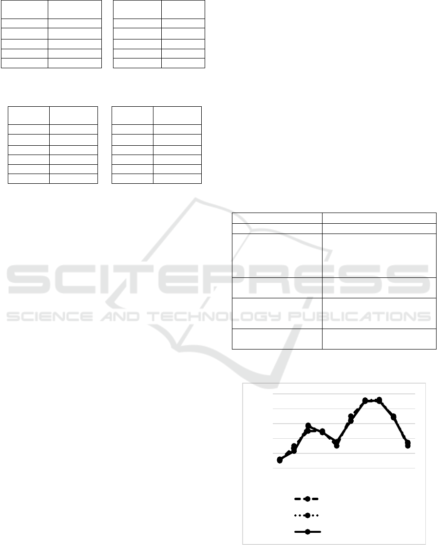
Table 4: GCV value based on uniform weighting for each
oscillation parameters.
Oscillation
Parameter
GCV
Value
Oscillation
Parameter
GCV
Value
1
164,001.8
33
6,317.85
2
145,905.457
34
6,041.737
3
116,867.687
35
5,880.609
4
103,764.306
36
5,910.787
37
7,320.536
Table 5: GCV value based on variance weighting for each
oscillation parameters.
Oscillation
Parameter
GCV
Value
Oscillation
Parameter
GCV
Value
1
19,680,216
33
776,253.6
2
17,508,654.9
34
732,082.2
3
14,024,122.4
35
712,005.9
4
12,451,716.7
36
708,797.7
5
10,386,213.6
37
1,591,221.6
38
1,663,382
It can be seen from Table 4, based on uniform
weighting obtained the minimum GCV is 5,880.609.
That value is achieved by the Fourier series
estimator with an oscillation parameter of 35. Table
5 shows the result that the minimum GCV value is
708,797.7 based on the variance weighting. That
value is achieved by the Fourier series estimator
with an oscillation parameter of 36. However, based
on the comparison of GCV values that be generated
in Table 4 and Table 5, it is seen that the GCV
values for uniform weighting is always smaller than
the GCV values for variance weighting in each
oscillation parameter. In this case, it can be
concluded that the uniform weighting is more
optimal than the variance weighting. However, this
study does not guarantee uniform weighting is
always better than variance weighting.
The selected of Fourier series estimator for
longitudinal data nonparametric regression approach
based on uniform weighting. The estimator has a
small MSE value of 0.00214. The estimator has a
high determination coefficient value of 0.99766
which means that predictors can explain the
response of 99.766%.
4.4 A Comparison
In this sub section we make comparison about the
result of regression for trend-seasonal data pattern
using linear estimator, the second estimator, and
Fourier series estimator, based on uniform
weighting. The comparison is presented on Table 6.
Based on Table 6, it should be noted that in the
goodness indicator of estimator, the Fourier series
estimator is better than the linear estimator for
regression that be used in case of trend – seasonal
longitudinal data pattern. The MSE for Fourier
series estimator is smaller than linear estimator. The
determination coefficient for Fourier series is greater
than linear estimator. In addition, the information
that be obtained based on the Fourier series
estimator is more complete than the linear estimator,
since the predictor that be contained in the model for
the Fourier series estimator are more complete.
Table 7 presents estimation result for both of
estimator for first subject. Based on Table 7 can be
inferred that estimator value for Fourier series is not
much different from the original data and linear
estimator. The result is supported by plot that be
presented on Figure 2. It can be concluded that
Fourier series estimator can become an alternative
for regression, in this case for longitudinal data.
Table 6: The comparison between linear and Fourier series
estimator in regression for trend-seasonal longitudinal data
pattern.
Linear estimator
Fourier series estimator
Consist of a predictor
Consist of two predictors
Does not fulfill the
assumption of
homogeneity
It does not test the
assumption of homogeneity,
because there has been no
relevant inference study.
MSE value equals to
0.1106
MSE value equals to0.00214
Determination
coefficient value
equals to 87.241%
Determination
coefficient value
equals to99.766%.
Estimator form is
parsimony
Estimator form is more
complex
Figure 2: Plot of the comparison result based on estimator
value from linear and Fourier series estimator and original
data for first subject.
2.85
2.95
3.05
3.15
3.25
3.35
1 2 3 4 5 6 7 8 9 10
y data
y linear
y Fourier series
Regression for Trend-Seasonal Longitudinal Data Pattern: Linear and Fourier Series Estimator
355

Table 7: The comparison based on estimator value from
linear and Fourier series estimator and original data for
first subject.
obs.
y data
y linear
y Fourier series
1
2.9
2.90543
2.910106
2
3
2.97832
2.964548
3
3.1
3.13808
3.132132
4
3.1
3.08934
3.090152
5
3
3.02323
3.027406
6
3.2
3.16562
3.170019
7
3.3
3.308
3.302801
8
3.3
3.31139
3.303712
9
3.2
3.19316
3.189406
10
3
3.0228
3.014211
5 CONCLUSIONS
In modelling longitudinal data with trend - seasonal
pattern with regression analysis, not only linear
estimators are used, but also the Fourier series
estimator can become an alternative. Based on the
discussion, the Fourier series estimator has better
value for the indicator of goodness estimator than
the linear estimator. The MSE for Fourier series
estimator is smaller than linear estimator. The
determination coefficient for Fourier series is greater
than linear estimator. Nevertheless, inference for the
Fourier series estimator still needs to be developed
ACKNOWLEDGEMENTS
The authors offer this paper to some institution that
give support to us, like University of Airlangga in
Surabaya, University of Gadjah Mada in
Yogyakarta, and Lembaga Pengelola Dana
Pendidikan (LPDP), part of The Ministry of Finance
in Indonesia, for scholarship that be received by
corresponding author throughout undergoes doctoral
program. For all the people who contribute to
support the completion of this paper, the authors
give high appreciation.
REFERENCES
Baltagi, B.H., 2005. Econometrics Analysis of Panel Data.
John Wiley and Sons Ltd. Chicester, 3
rd
edition.
Bilodeau, M., 1992. Fourier Smoother and Additive
Models. The Canadian Journal of Statistics, 3,
257-269.
Bloomfield, P., 2000. An Introduction Fourier Analysis
for Time Series. John Wiley and Sons Inc. New York.
Box, G. E. P., Jenkins, G. M., and Reinsel, G. C., 1976.
Time Series Analysis: Forecasting and Control. John
Wiley and Sons, Inc. New York.
Budiantara, I. N., Ratnasari, V., Zain, I., Ratna, M., and
Mardianto, M. F. F., 2015. Modeling of HDI and
PQLI in East Java (Indonesia) using Biresponse
Semiparametric Regression with Fourier Series
Approach. ATABS Journal, 5(4), 21–28.
Greene, W. H., 2012. Econometric Analysis. Prentice Hall
International. New Jersey, 7
th
Edition.
Gujarati, D. N., 2004. Basic Econometrics. The Mc. Grew
Hill Companies. New York, 4
th
Edition.
Hardle, W., 1990. Applied Nonparametric Regression.
Cambridge University Press. New York.
Wu, H., and Zhang, J. T., 2006. Nonparametric
Regression Methods for Longitudinal Data Analysis.
John Wiley and Sons, Inc. New Jersey.
Takezawa, K., 2006. Introduction to Nonparametric
Regression. John Wiley and Sons, Inc. New Jersey.
Tripena, A., and Budiantara, I. N., 2006. Fourier Estimator
in Nonparametric Regression. Proceeding
International Conference on Natural Sciences and
Applied Natural Scienes Ahmad Dahlan University,
Yogyakarta.
Wu, H., and Zhang, J. T., 2006. Nonparametric
Regression Methods for Longitudinal Data Analysis.
John Wiley and Sons, Inc, New Jersey.
ICMIs 2018 - International Conference on Mathematics and Islam
356
