
Air Pollution Prediction with Hotspot Variable based on Vector
Autoregressive Model in Pekanbaru Region
Ari Pani Desvina
1
, Arinal Haque
1
, Riswan Efendi
1
, Muspika Hendri
2
,
Mas’ud Zein
2
and Sri Murhayati
2
1
Department of Mathematics, Faculty of Sciences and Technology, Universitas Islam Negeri Sultan Syarif Kasim Riau,
Indonesia
2
Faculty of Trainer Teacher and Education, Universitas Islam Negeri Sultan Syarif Kasim Riau, Indonesia
sri.murhayati}@uin-suska.ac.id
Keywords: Particulate Matter (PM10), Vector Autoregressive (VAR) Model.
Abstract: The air quality is widely caused by pollution of particulate matter (PM10) and meteorological elements. For
examples, rainfall, solar radiation, air temperature, humidity, wind velocity, and hotspot. In analysis data
(ADV), the used variables are more than one variable, so that the best model for modeling and forecasting
multivariate data is vector autoregressive (VAR). The VAR model is chosen because it is one of multivariat
analysis for time series data and it is able to describe the interconnectedness among variables. The aim of this
research is to find the best model for PM10 concentrations with other meteorological elements in Pekanbaru
by using VAR model, and to determine the prediction result of PM10 concentration in the future. Furthermore,
the monthly data of Pekanbaru region from January 2011 until December 2015 was used for training and
testing. The result showed the best model for predicting PM10 is VAR(1). It can be summarized that rainfall,
solar radiation, humidity and hotspot variables have been interconnected with PM10. Based on proposed
model, the concentration of PM10 data increased from January 2016 until December 2017.
1 INTRODUCTION
Air is a very important factor for all substance’s life
in the earth. It has created by God (Allah SWT) with
the sidelines of the wind, as described in the Qur'an
Surah Ar-Ruum (48) is “God is He who sends the
winds. They stir up clouds. Then He spreads them in
the sky as He wills. And He breaks them apart. Then
you see rain drops issuing from their midst. Then,
when He makes it fall upon whom He wills of His
servants, behold, they rejoice”.
In this decade, the city centers development such
as the technological advancements have been raised
fast which may influence the air quality negatively.
Furthermore, the existence of city center
development, the number of plant construction, and
the number of new lands opening by companies with
burning method will produce the air conditions
become dry and dirty. Additionally, the increasing
number of motor vehicles also resulted in increased
density in traffic so that the quality of the air even
more alarming. As explained in the Qur'an Surat Al-
A'raf in verse (56) explains about Allah’s prohibition
to damage the environment to man, because Allah
will give a bigger penalty, but man still deny it, as for
verse (56) in surah Al-A'raf is “And do not corrupt on
earth after its reformation and pray to Him with fear
and hope. God’s mercy is close to the doers of good”.
Air pollution is the presence of chemicals in the
air which certain characteristics and periods of time
whose effects can cause dangerous condition to
human body, animal and plant. The prominent
substances of air pollution are carbon monoxide,
carbon dioxide, nitrogen oxide, nitrogen dioxide,
particulate matter (PM
10
) and the other components.
Particulate matter (PM
10
) is microscope which
diameter is less than 10 µm and it is able to cause a
serious effect on human health risks, animal and plant
than other larger components, generally it is a result
from forest and land burning illegally (Strauss et al,
1984).
In 2015, burning forest and opening land for
agriculture had happened in Riau province, so the
number of hotspots is very high, it is resulting in high
concentration of air pollutant gas such as particulate
Desvina, A., Haque, A., Efendi, R., Hendri, M., Zein, M. and Murhayati, S.
Air Pollution Prediction with Hotspot Variable based on Vector Autoregressive Model in Pekanbaru Region.
DOI: 10.5220/0008521403190327
In Proceedings of the International Conference on Mathematics and Islam (ICMIs 2018), pages 319-327
ISBN: 978-989-758-407-7
Copyright
c
2020 by SCITEPRESS – Science and Technology Publications, Lda. All rights reserved
319

matter (PM10). Therefore, there was air pollution in
various regions in Riau Province and even in the areas
outside of Riau. In addition to causing illness, fog
smoke in Riau, especially in Pekanbaru causes
community activities disturbed, such as all education
activities in Riau, especially Pekanbaru City have
been stopped. One of the universities which halts its
academic activities, for 4 days, was the State Islamic
University of Sultan Syarif Kasim Riau. Moreover,
the visibility on the highway is only ± 200 meters,
thus causing rider activity is hampered. Air pollution
by particulate matter (PM10) has a dynamic
relationship with meteorological elements such as
rainfall, solar radiation, air temperature, humidity and
wind speed. In addition, the number of hotspots also
has a dynamic relationship with air pollution caused
by particulate matter (PM10) (Brown and Davis, 1973).
The guidance of Allah SWT about the duty of His
people to be grateful for the blessings that Allah
Almighty gives which is much explained in the
Qur'an, including the favor of the universe that Allah
has created for His people. Allah SWT asserted in
Qur'an that is for His people who are not grateful for
the blessings that Allah Almighty gives, then Allah
SWT will give a very painful penalty, which is
described in surah Ibrahim verse 7 is “And when your
Lord proclaimed: “If you give thanks, I will grant you
increase; but if you are ungrateful, My punishment is
severe”.
Several studies related to the study of air pollution
modeling and number of hotspots using vector
autoregressive (VAR) models have been conducted
by, such as a research conducted by Cai (2008) used
VAR analysis to predict the time series data of CO
pollution in California. Another research is Ahmad,
et al (2013) discusses the prediction of air pollution
by particulate matter (PM10) using the Box-Jenkins
method. Based on the explanation of air pollution, it
is necessary to predict the concentration of air
pollutant that is especially gas particulate matter
(PM10) and relating elements for the future by using
vector autoregressive model (VAR). Given the
importance of knowing the concentration of particle
matter (PM10) in Pekanbaru, this research tries to
provide a suitable statistical model for particulate
matter (PM10) data in Pekanbaru by using vector
autoregressive model (VAR). The purpose of this
research is to find the best model for particulate
matter density data (PM10) along with
meteorological elements in Pekanbaru city by using
vector autoregressive model (VAR). And determine
the prediction result of particulate matter
concentration (PM10) in the future by using vector
autoregressive (VAR) model in Pekanbaru city.
2 METHODS
2.1 Literature Review
Particulate matter (PM10) is particles which diameter
is less than 10 µm which can cause more hazardous
effect on human health, animal and plant than some
other larger particles formed of stationary source such
as vehicles (vehicle ekzos). Particulate Matter
(PM10) is largely produced from wild forest and land
burning. Rainfall is the height of rainwater collected
in a flat, non-volatile, non-pervasive and non-flowing
place (Chelani et al, 2004).
Solar radiation is energy radiance which comes
from thermonuclear process in the sun. Solar energy
is the energy source for all of existence. The air
temperature is a measure of the average kinetic
energy of molecule improvements or the temperature
condition of the air. The hotspot is the terminology of
a single pixel that has a higher temperature than the
surrounding area or location captured by a digital data
satellite sensor. Air humidity is the amount of water
vapor in the air (atmosphere) at a given time and
place. Wind is the air movement parallel to the
surface of the earth. Air moves from high pressure
areas to low pressure areas (Liew, 2002).
Prediction or forecasting is a forecasting process
for the future based on past data. Forecasting is a
fundamental thing in determining a plan or policy in
an agency this is due to the uncertainty of the values
of a variable in the future. Therefore, predictions are
very important in many fields because predictions of
future events must be incorporated into the process of
making a decision. The definition of the VAR model
is that all variables present in the VAR model are
endogenous. If there is a relationship associate
between variables observed, then the variables need
to be done the same way. So, there is no longer
endogenous and exogenous variables (Bowerman et
al, 2005). In general, the model VAR lag p for n
variables can be formulated as follows (Makridakis,
1998):
with
1
,
tt
YY
is a vector which size is
1n
containing
n
variables entered in the VAR model at t time and
t – 1, i = 1,2,…, p,
is a vector of intercept which
size is n × 1,
is a coefficient matrix of sizes n × n
for each, , i = 1,2,…, p,
is a vector of sized n × 1
that is
,
p
is lag VAR, t is a period
of observation. The VAR model consisting of two
variables and 1 lag is the VAR(1) model:
ICMIs 2018 - International Conference on Mathematics and Islam
320

According Makridakis et.al (1998), the VAR
model advantage is the researchers do not need to
distinguish which endogenous and exogenous
variables because all variables VAR is endogenous.
The method of estimation is simple with the least
squares method and can be made in separate model
for each endogenous variable. Assumptions that must
be met from the times series data to form the VAR
model are stationary and independence error (error no
autocorrelation).
2.2 Data and Research Methodology
The data of air pollution especially particulate matter
parameter (PM10) was obtained from the Pekanbaru
Environmental station. Meteorological elements such
as solar radiation, air temperature, rainfall, humidity
and wind speed are obtained from the Meteorology,
Climatology and Geophysics (BMKG) station of
Pekanbaru, while the data of the number of hotspots
(hotspots) obtained from the Center for Natural
Resources Conservation Pekanbaru. The data used in
this research are the monthly data of air pollution data
which parameter particulate matter (PM10), rainfall,
solar radiation, air temperature, humidity and wind
speed, hotspot number are from 2011 to 2015. The
calculation method used in this research is the method
of completion based on the formulas of vector
autoregressive model (VAR), then applied into the
form of EVIEWS and Minitab programming.
2.3 Steps in Forming VAR Model
2.3.1 Data Stationary Test
A data is said to be stationary if the data has a variance
that is not too large and has a tendency to approach
the average value (Bierens, 2006). There are many
ways that can be used to test the stationary data in
time series analysis i.e. see the plot of actual data, see
plot ACF and PACF is the actual data plot and plot
ACF and PACF is said to stationary if the plot of
actual data has average traits and variance which is
constant all the time and on ACF plots and PACF
plots drop exponentially. Stationary or not stationary
data can be tested by running statistical tests i.e. unit
root test. There are several statistical tests that can be
used to determine the stationary or not stationary. The
most commonly used tests are Augmented Dickey
Fuller (ADF), Phillips Perron (PP) and Kwiatkowski
Phillips Schmidt Shin (KPSS) tests (Bierens, 2006).
2.3.2 The Determination of Lag VAR
The lag determination is used to determine the
optimal lag length to be used in further analysis and
will determine the parameter estimate for the VAR
model. According to Bierens (2006) that the VAR lag
can be determined using AIC (Akaike Information
Criterion), SIC (Schwarz Information Criterion) and
HQ (Hannan-Quinn Information Criterion). AIC, SIC
and HQ measure the validity of the model that
improves the loss of degrees freedom when additional
lags are included in the model. Lag VAR is
determined by the lag value that results in the smallest
AIC, SIC and HQ (Bierens, 2006).
2.3.3 Granger Causality Test
The Granger causality test is a test that can be used to
analyze the causality relationship between the
observed variables. The Granger causality test is used
to look at the direction of the relationship between the
variables (Vandaele, 1983).
2.3.4 The Estimation and Forecasting of
VAR
A simple VAR consisting of two variables and 1 lag
can be formulated into both equations. The
parameters in the VAR model can be estimated by
using the maximum likelihood by minimizing the
derivative function of the VAR model parameters by
minimizing the sum of the error squares for the VAR
model equations (Brocklebank & David, 2003).
2.3.5 VAR Model Assumption Test
After the VAR model is obtained then the Lagrange
Multiplier (LM) is tested by looking at the value of
Q-statistics and Chi-square (Chatfield, 2003).
2.3.6 The Forecasting for Future Time
The next step in the VAR model is prediction. The
VAR model formed from data is used to make
predictions that include training and predictions for
the future. Training prediction stage, the data used is
the first actual until the last actual data. Furthermore,
at the prediction stage for the time to come, the data
used is the final data from the actual data (Chatfield,
2003).
Air Pollution Prediction with Hotspot Variable based on Vector Autoregressive Model in Pekanbaru Region
321
3 RESULTS AND DISCUSSIONS
The Statistika Descriptive of Data Research
Descriptive statistics for particulate matter
concentration (PM10), rainfall, solar radiation, air
temperature, humidity, wind speed, and hotspots were
observed on a monthly basis for five years, from 2011
to 2015. All data for all variables experience an
increasing and decreasing for each month, for the
mean, median, maximum value, minimum value and
standard deviation can be seen in the following table:
Table 1: Descriptive Statistics PM10, Rainfall, Solar
Radiation, Air Temperature, Air Humidity, Wind Speed,
and Hotspot.
Variable
PM10
Rainfall
Solar
Radiation
Mean
48.43
202.8
46.40
Median
27.96
184.2
50.00
Maximum
310.31
313
57
Minimum
20.38
11.1
7
Standard
Deviation
9.28
123.9
14.08
Observasi (N)
60
60
60
Variable
Air
Temperature
Air
Humidity
Wind Speed
Mean
27.135
77.467
5.5500
Median
27.200
78.000
5.8000
Maximum
27.6
80
6
Minimum
25.3
69
3.7
standard
Deviation
0.646
3.762
0.6105
Observasi (N)
60
60
60
Variable
Hotspot
Mean
331.0
Median
185.0
Maximum
438.8
Minimum
3
standard
Deviation
376.9
Observasi (N)
60
The Formation of Prediction Model Particulate
Matter 10 (PM10) by using Vector Autoregressive
Model (VAR)
An autoregressive vector model (VAR) in formed for
the prediction of air pollution data by particulate
matter (PM10) and meteorological elements must
follow several steps: data validation test, determine
optimal lag length of vector autoregressive model
(VAR), granger causality test, vector autoregressive
model parameters (VAR), test of autoregressive
vector model (VAR), and data prediction for the
future. Data used in this research are data particulate
matter (PM10), rainfall, solar radiation, air
temperature, humidity, wind speed (wind speed), and
hotspot (hotspot). The data used is time series data
from January 2011 to December 2015. Therefore, the
amount of data is 60 data.
Stage 1: The Stationary Data Test
Initial step in processing time series data by using
vector autoregressive model (VAR) to predict the
time data that will come is a stationary data test. In
data processing, we use Minitab and Eviews software.
The stationary data test can be analyzed from the plot
of actual data, plot autocorrelation function (ACF)
and partial autocorrelation function (PACF), and unit
root test. In the test phase of the stationary data test
can be analyzed from the actual data plot of
particulate matter (PM10), rainfall, solar radiation, air
temperature, air humidity, wind speed and hotspot
with 60 observations from January 2011 to December
2015:
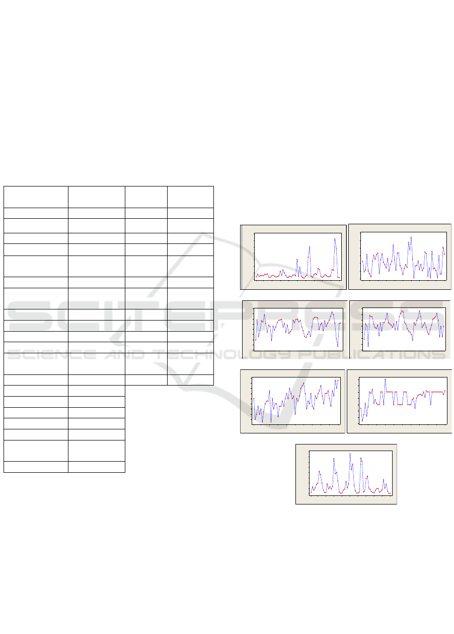
(a) (b)
(c) (d)
(e) (f)
(g)
Figure 1: Time series plot for (a) PM10 concentration, (b)
rainfall, (c) solar radiation, (d) air temperature, (e) air
humidity, (f) wind speed, (g) hotspot in Pekanbaru City.
Based on Figure 1, the graph of particulate matter
(PM10), rainfall, solar radiation, air temperature, air
humidity, wind speed and hotspot of Pekanbaru
shows that all data on all variables meet the
requirements of the stationary data test because the
data averages and variants move constantly over time.
Month
PM10
60544842363024181261
350
300
250
200
150
100
50
0
Time Series Plot of PM10
Month
Rainfall
60544842363024181261
600
500
400
300
200
100
0
Time Series Plot of Rainfall
Month
Solar Radiation
60544842363024181261
80
70
60
50
40
30
20
10
0
Time Series Plot of Solar Radiation
Month
Air Temperature
60544842363024181261
28,5
28,0
27,5
27,0
26,5
26,0
25,5
25,0
Time Series Plot of Air Temperature
Month
Air Humadity
60544842363024181261
86
84
82
80
78
76
74
72
70
Time Series Plot of Air Humadity
Month
Wind Speed
60544842363024181261
7,0
6,5
6,0
5,5
5,0
4,5
4,0
3,5
Time Series Plot of Wind Speed
Month
HOTSPOT
60544842363024181261
1600
1400
1200
1000
800
600
400
200
0
Time Series Pl ot of HOTS POT
ICMIs 2018 - International Conference on Mathematics and Islam
322
Data stationary can also be viewed through the plot of
autocorrelation function (ACF) and partial
autocorrelation function (PACF). Plot ACF and
PACF plot can be seen Figure 2 below:
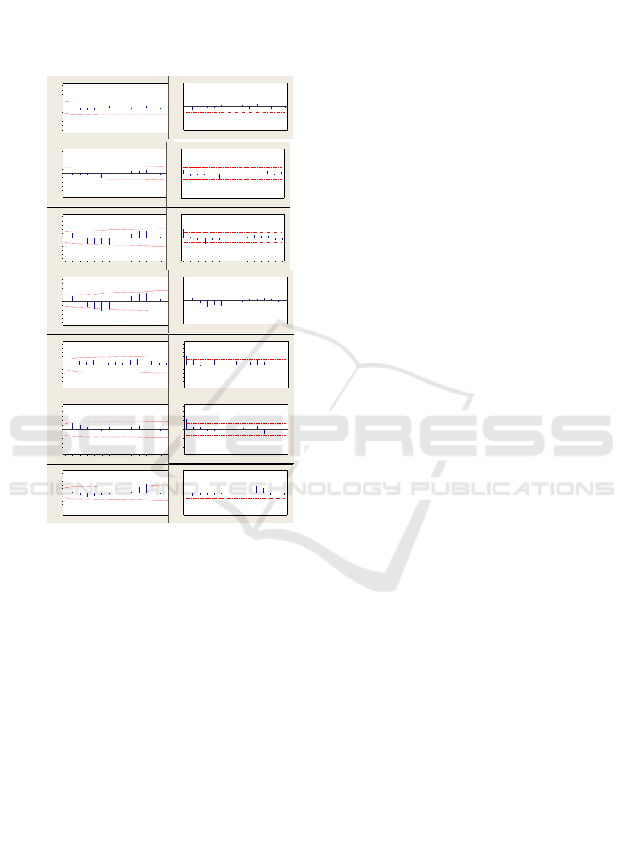
(a)
(b)
(c)
(d)
(e)
(f)
(g)
ACF
PACF
Figure 2: ACF and PACF Plots for (a) PM10 concentration,
(b) rainfall, (c) solar radiation, (d) air temperature, (e) air
humidity, (f) wind speed, (g) hotspot in Pekanbaru City.
Figure 2 shows that the data particulate matter
(PM10), rainfall, solar radiation, air temperature, air
humidity, wind speed and hotspot of Pekanbaru have
been said to tend to be stationary due to each lag on
the ACF plot shrinks towards zero exponentially and
PACF shows that its value is truncated to a certain
lag. based the two graphs above, the stationary data
test can be also through unit root test. The root unit
test has been tested using three test types: Augmented
Dickey Fuller (ADF), Phillips Perron (PP), and
Kwiatkowski Phillips Schmidt Shin (KPSS) tests.
The following will be a unit root test for data
particulate matter (PM10), rainfall , solar radiation,
air temperature, humidity, wind speed (wind speed),
and hotspot (hotspot) of Pekanbaru.
Hypothesis testing for ADF test used for data
particulate matter (PM10), rainfall, solar radiation, air
temperature, air humidity, wind speed and hotspot are
0:
Ho
; that there are root unit (non-stationary
data) versus
0:1
H
; that is there is no root unit
(stationary data). Hypothesis testing for PP test is
0:
Ho
, there is unit root (data not stationary), the
opponent is
0:1
H
, there is no root unit (stationary
data). KPSS test has the hypothesis testing
0:
Ho
, there is no root unit (stationary data), and the
opponent is
0:1
H
, there is unit root (data not
stationary). Test results of PM10 data, rainfall, solar
radiation, air temperature, air humidity, wind speed
and hotspot using unit root test of ADF, PP and KPSS
can be presented in Table 2.
Table 2 shows that all variables have
> absolute
value for MacKinnon critical value at a significant
level of 0.05 or can be seen from the p-value which
all p-values in all variables are less than significant
0.05 then decline
Ho
, that PM10 data, rainfall, solar
radiation, air temperature, air humidity, wind speed
and hotspot do not have root unit, this means that time
series for PM10 data, rainfall, radiation sun, air
temperature, air humidity, wind speed (wind speed),
and hotspot is stationary.
Stage 2: The Determination of the Optimal Lag
Length
Data particulate matter (PM10), rainfall, solar
radiation, air temperature, air humidity, wind speed,
and hotspot (fire point) are stationary, the next step is
to determine the optimal lag length that will be used
in autoregressive vector model (VAR). Based on
Eviews software, it is obtained the optimal lag length
as in Table 3. In Table 3 can be seen that the values
of AIC, SC, and HQ which are asterisks and the
smallest among the lags of zero to the third lag are
AIC in lag 1. So, we can know that the optimal lag
used for the vector autoregressive (VAR) model is on
the lag 1 or VAR(1) model.
Stage 3: The Causality of Granger Test
After the optimal lag length is obtained, the next step
is to test the granger causality. Granger causality test
is performed to see whether or not a direct or
reciprocal relationship between variables. The
following results of granger causality test using
Eviews software can be presented in Table 4.
Lag
Autocorrelation
151413121110987654321
1,0
0,8
0,6
0,4
0,2
0,0
-0,2
-0,4
-0,6
-0,8
-1,0
ACF Plot of PM1 0
Lag
Partial Autocorrelation
151413121110987654321
1,0
0,8
0,6
0,4
0,2
0,0
-0,2
-0,4
-0,6
-0,8
-1,0
PACF Plot of PM10
Lag
Autocorrelation
151413121110987654321
1,0
0,8
0,6
0,4
0,2
0,0
-0,2
-0,4
-0,6
-0,8
-1,0
ACF Plot of Rainfall
Lag
Partial Autocorrelation
151413121110987654321
1,0
0,8
0,6
0,4
0,2
0,0
-0,2
-0,4
-0,6
-0,8
-1,0
PACF Plot of Rainfall
Lag
Autocorrelation
151413121110987654321
1,0
0,8
0,6
0,4
0,2
0,0
-0,2
-0,4
-0,6
-0,8
-1,0
ACF Plot of Solar Radiation
Lag
Partial Autocorrelation
151413121110987654321
1,0
0,8
0,6
0,4
0,2
0,0
-0,2
-0,4
-0,6
-0,8
-1,0
PACF Plot of Solar Radiation
Lag
Autocorrelation
151413121110987654321
1,0
0,8
0,6
0,4
0,2
0,0
-0,2
-0,4
-0,6
-0,8
-1,0
ACF Plot of Air Temperature
Lag
Partial Autocorrelation
151413121110987654321
1,0
0,8
0,6
0,4
0,2
0,0
-0,2
-0,4
-0,6
-0,8
-1,0
PACF Plot of Air Temperature
Lag
Autocorrelation
151413121110987654321
1,0
0,8
0,6
0,4
0,2
0,0
-0,2
-0,4
-0,6
-0,8
-1,0
ACF Plot of Air Humadi ty
Lag
Partial Autocorrelation
151413121110987654321
1,0
0,8
0,6
0,4
0,2
0,0
-0,2
-0,4
-0,6
-0,8
-1,0
PACF Plot of Air Humadi ty
Lag
Autocorrelation
151413121110987654321
1,0
0,8
0,6
0,4
0,2
0,0
-0,2
-0,4
-0,6
-0,8
-1,0
ACF Plot of Wind S peed
Lag
Partial Autocorrelation
151413121110987654321
1,0
0,8
0,6
0,4
0,2
0,0
-0,2
-0,4
-0,6
-0,8
-1,0
PACF Plot of Wind S peed
Lag
Autocorrelation
151413121110987654321
1,0
0,8
0,6
0,4
0,2
0,0
-0,2
-0,4
-0,6
-0,8
-1,0
ACF Plot of Hotspot
Lag
Partial Autocorrelation
151413121110987654321
1,0
0,8
0,6
0,4
0,2
0,0
-0,2
-0,4
-0,6
-0,8
-1,0
PACF Plot of Hotspot
Air Pollution Prediction with Hotspot Variable based on Vector Autoregressive Model in Pekanbaru Region
323

Table 2: ADF, PP, and KPSS Test Value Compared with
MacKinnon Critical Values for PM10 Data of Pekanbaru
City.
Variable
ADF
p-value
t-stat
t-critical
MacKinnon (5%)
PM10
0.0001
-4.96
-2.912
Rainfall
0.000
-6.26
-2.912
Solar
Radiation
0.0001
-5.11
-2.912
Air
Temperature
0.000
-5.39
-2.916
Air Humidity
0.0145
-3.57
-2.913
Wind speed
0.0004
-4.59
-2.912
Hotspot
0.0004
-4.60
-2.912
Variable
PP
p-value
t-stat
t-critical
MacKinnon (5%)
PM10
0.0004
-4.64
-2.912
Rainfall
0.000
-6.16
-2.912
Solar
Radiation
0.0001
-5.16
-2.912
Air
Temperature
0.000
-5.35
-2.912
Air Humidity
0.0006
-4.47
-2.912
Wind speed
0.0006
-4.49
-2.912
Hotspot
0.0009
-4.37
-2.912
Variable
KPSS
t-stat
t-critical MacKinnon (5%)
PM10
0.335
0.463
Rainfall
0.089
0.463
Solar
Radiation
0.077
0.463
Air
Temperature
0.053
0.463
Air Humidity
0.087
0.463
Wind speed
0.370
0.463
Hotspot
0.186
0.463
Table 3: The Optimal Lag length.
Lag
AIC
SC
HQ
0
52.75358
53.00448*
52.85109
1
52.05960*
54.06681
52.83967*
2
52.22299
55.98650
53.68562
3
52.35758
57.87741
54.50278
Table 4: The Causality of Granger Test.
No
Hipotesis
Obs
F-Statistik
P-Value
1
WS not affect RF
RF not affect WS
59
0.53571
2.03996
0.4673
0.1588
2
AH not affect RF
RF not affect AH
59
0.0000063
0.00663
0.9980
0.9354
3
PM10 not affect RF
RF not affect PM10
59
0.04065
0.23779
0.8409
0.6277
4
SR not affect RF
RF not affect SR
59
5.07833
1.30892
0.0282
0.2575
5
AT not affect RF
RF not affect AT
59
0.12241
0.03840
0.7277
0.8454
6
HP not affect RF
RF not affect HP
59
0.16547
1.26958
0.6857
0.2647
7
AH not affect WS
WS not affect AH
59
0.01387
6.04835
0.9067
0.0170
8
PM10 not affect WS
WS not affect PM10
59
0.53467
0.44312
0.4677
0.5084
9
SR not affect WS
WS not affect SR
59
3.37422
0.18205
0.0715
0.6713
10
AT not affect WS
WS not affect AT
59
5.51941
0.31647
0.0224
0.5760
11
HP not affect WS
WS not affect HP
59
0.54855
0.88732
0.4620
0.3503
12
WS not affect RF
RF not affect WS
59
0.53571
2.03996
0.4673
0.1588
13
AH not affect RF
RF not affect AH
59
0.0000063
0.00663
0.9980
0.9354
14
PM10 not affect RF
RF not affect PM10
59
0.04065
0.23779
0.8409
0.6277
15
SR not affect RF
RF not affect SR
59
5.07833
1.30892
0.0282
0.2575
16
AT not affect RF
RF not affect AT
59
0.12241
0.03840
0.7277
0.8454
17
HP not affect RF
RF not affect HP
59
0.16547
1.26958
0.6857
0.2647
18
AH not affect WS
WS not affect AH
59
0.01387
6.04835
0.9067
0.0170
19
PM10 not affect WS
WS not affect PM10
59
0.53467
0.44312
0.4677
0.5084
20
SR not affect WS
WS not affect SR
59
3.37422
0.18205
0.0715
0.6713
21
AT not affect WS
WS not affect AT
59
5.51941
0.31647
0.0224
0.5760
22
HP not affect WS
WS not affect HP
59
0.54855
0.88732
0.4620
0.3503
where PM10 is particulate matter 10, RF is rainfall,
SR is solar radiation, AT is air temperatur, AH is air
humidity, WS is wind speed, and HP is hotspot.
Base on table 4, it is obtained the result of
Granger’s causality test as:
Granger’s causality test, wind speed and rainfall :
a.
: wind speed doesn’t affect rainfall
: wind speed affects rainfall
Rejection area: if p-value < α then H
0
is rejected,
otherwise if P-value ≥ α then H
0
is accepted.
Based on the test results obtained that the P-value
≥ α is 0.4673 ≥ 0.05. This means that H
0
is
ICMIs 2018 - International Conference on Mathematics and Islam
324

accepted so that wind speed does not affect
rainfall.
b.
: Rainfall doesn’t affect wind speed
: Rainfall affects wind speed
Rejection area: if P-value <α then H
0
is rejected,
otherwise if P-value ≥ α then H
0
is accepted.
Based on the test results obtained that the P-value
≥ α is 0.1588 ≥ 0.05. This means that H
0
is
accepted so that rainfall does not wind speed.
For Granger Causality testing no. 2-21 may be
carried out in the same manner in the test above.
Based on the Granger Causality test before, it can be
seen that who has causality between variables i.e.
solar radiation affects rainfall, wind velocity affects
air humidity, air temperature affects wind speed,
PM10 affects the amount of hotspot and solar
radiation affects air temperature. So, it can be
concluded that the elements of rainfall, solar
radiation, air temperature, and hotspots have a
relationship to PM10.
Stage 4: Parameter Estimation
This step is a parameter estimating step for the VAR
model. In the second step, it has obtained the length
of the lag is 1 which consists of 7 variables so that the
resulting model to be estimated is VAR(1). The
VAR(1) model can be :
10 11 1 12 1 13 1 14 1
15 1 16 1 17 1
t t t t t
t t t
PM PM RF SR AT
AH WS HP
(1)
20 21 1 22 1 23 1 24 1
25 1 26 1 27 1
t t t t t
t t t
RF PM RF SR AT
AH WS HP
(2)
30 31 1 32 1 33 1 34 1
35 1 36 1 37 1
t t t t t
t t t
SR PM RF SR AT
AH WS HP
(3)
40 41 1 42 1 43 1 44 1
45 1 46 1 47 1
t t t t t
t t t
AT PM RF SR AT
AH WS HP
(4)
50 51 1 52 1 53 1 54 1
55 1 56 1 57 1
t t t t t
t t t
AH PM RF SR AT
AH WS HP
(5)
60 61 1 62 1 63 1 64 1
65 1 66 1 67 1
t t t t t
t t t
WS PM RF SR AT
AH WS HP
(6)
70 71 1 72 1 73 1 74 1
75 1 76 1 77 1
t t t t t
t t t
HP PM RF SR AT
AH WS HP
(7)
The result of parameter estimation is obtained using
Eviews software. The results of the VAR(1) model
parameter estimation are presented in equations
below. The model parameters can be substituted into
the VAR(1) model using equations (1), (2), (3), (4),
(5), (6), and (7):
1 1 1
1 1 1 1
149.738 0.4162 0.0524 0.9364
12.9010 2.4060 1.5020 0.0048
t t t t
t t t t
PM PM RF SR
AT AH WS HP
(8)
1 1 1
.
1 1 1 1
995.588 0.4290 0.1336 5.8629
60.1550 5.8621 52.4149 0.0175
t t t t
t t t t
RF PM RF SR
AT AH WS HP
(9)
1 1 1
1 1 1 1
197.372 0.0975 0.0367 0.0553
6.1958 0.9911 1.3836 0.0040
t t t t
t t t t
SR PM RF SR
AT AH WS HP
(10)
111
1 1 1 1
22.301 0.0004 0.0003 0.0206
0.1089 0.0254 0.1762 0.0000067
t t t t
t t t t
AT PM RF SR
AT AH WS HP
(11)
1 1 1
1 1 1 1
33.1204 0.0265 0.0058 0.02105
0.501 0.2323 1.8505 0.00276
t t t t
t t t t
AH PM RF SR
AT AH WS HP
(12)
1 1 1
1 1 1 1
3.85 0.0015 0.00044 0.0085
0.1772 0.0282 0.372 0.0000758
t t t t
t t t t
WS PM RF SR
AT AH WS HP
(13)
1 1 1
1 1 1 1
.
2144.33 2.565 0.877 0.4899
35.0203 28.342 101.849 0.6747
t t t t
t t t t
HP PM RF SR
AT AH WS HP
(14)
Stage 5: Verification of VAR Model
When the model for prediction is obtained, VAR(1),
it needs to verification by using test Lagrange
Multiplier Test (LM test). This verification is done by
checking whether the residual correlated or not by
using Lagrange Multiplier test (LM test), this test is
using Eviews software. The hypothesis testing of the
Lagrange Multiplier test is H
0
: There is no significant
autocorrelation to the h-lag (feasible model) versus
H1: There is significant autocorrelation to the h-lag
(improper model). By using a significant level, it can
be determined a criterion which is if the p-value >
, H
0
is accepted which means there is no significant
autocorrelation component until lag h or feasible
model. Vice versa if the p-value
then H
0
is
rejected, which means there is a significant
autocorrelation component until the h lag or model is
not feasible. Table 5 is the result of Lagrange
Multiplier test.
Based on Table 5 above, it is found that all p-
values exceed the significant or p-value >
for all
lags or up to twelve lags. This means that there is no
Air Pollution Prediction with Hotspot Variable based on Vector Autoregressive Model in Pekanbaru Region
325
significance component at 5% alpha, all p-values in
each lag greater than 0.05 indicate that no
autocorrelation or model error exists.
Table 5: The Result of Lagrange Multiplier Test (LM Test).
Lags
LM-Stat
Prob
Lags
LM-Stat
Prob
1
65.00721
0.0625
7
46.15437
0.5892
2
56.12147
0.2255
8
50.94637
0.3969
3
62.02264
0.1002
9
43.65337
0.6890
4
50.83375
0.4012
10
31.50254
0.9754
5
50.50584
0.4138
11
57.62338
0.1864
6
41.54211
0.7664
12
55.25166
0.2504
Stage 7: Application of Models for Forecasting
After running the goodness model test using the LM
test, which states that the VAR(1) model is feasible to
be used for prediction in the future and after
performing prediction for data training and data
testing, further predictions are made for future time
on particulate matter (PM10) and hotspots. Prediction
of particulate matter concentration (PM10) and
hotspot data begins from January 2016 to December
2017. The prediction result of particulate matter
(PM10) and hotspot can be presented in the following
graph:
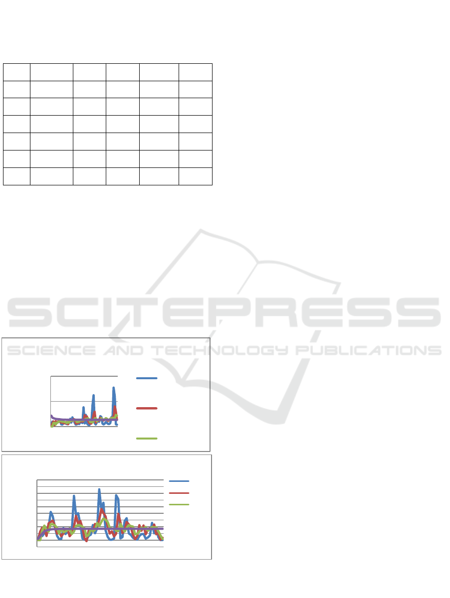
Figure 3: Graph of Actual Data, Training, Testing, and
Prediction Data for PM10 (above) and Hotspot Data
(below) from January 2016 to December 2017.
Based on Figure 3 we can see that the prediction
results of particulate matter (PM10) of Pekanbaru
from January 2016 to December 2017 experienced a
slight decreased from the previous month in 2016
until 2017. As for the prediction of Riau’s hotspot
data (hotspots) from January 2016 to December 2017
experienced a slight increase from the previous
months.
4 CONCLUSIONS
In this paper, we obtained the prediction model for
particulate matter (PM10) with some external
variable (vector), namely, the rainfall, the solar
radiation, the air temperature, the air humidity, the
wind speed and the hotspot. Mathematically has been
explained in the Equation (15). By using this equation
(model), the prediction of air pollution (data training)
can be achieved closely with their actual data.
Additionally, these also occurred with prediction of
the meteorological particles. While, the data testing is
not fully achieved using proposed model for both data
sets. Thus, the prediction of PM10 has been decreased
from January 2016 until December 2017 at Pekanbaru
region. On the other hands, the hotspot prediction was
almost same with their actual data from the same
period. From Granger test, some external vector
above also contributed potentially to PM10.
ACKNOWLEDGEMENTS
We would like to thank the Head of Pekanbaru
Environmental station, Head of Meteorology,
Climatology and Geophysics (BMKG) station of
Pekanbaru and Head of Pekanbaru City Natural
Resources Conservation Center, which has provided
assistance to us to get air pollution data and
meteorological elements and hotspots in Pekanbaru.
REFERENCES
Ahmad, M & Pani, A. D., 2013. Time Series Analysis of
Particulate Matter (PM10) in Klang Valley, Malaysia.
Journal of Quality Measurement and Analysis. Vol. 9
No. 1. July 2013. 65-80.
Bierens, H. J., 2006. Information Criteria and Model
Selection. Pennsylvania. Pennsylvania State
University.
Bowerman, B. L., O’Connell, R. T. & Koehler, A. B., 2005.
Forecasting, Time Series, Regression an applied
-200
0
200
400
600
800
1000
1200
1400
1600
1800
1 4 7 10 13 16 19 22 25 28 31 34 37 40 43 46 49 52 55 58
Hotspot
Graph of Actual Data, Training, Testing, and Prediction for Hotspot Data
Actual
Data
Training
Testing
Month
0
200
400
1 101928374655
PM10
Graph Actual Data, Training, Testing, and
Prediction for Particulate Matter 10 Data
Actual
Data
Training
Testing
Month
ICMIs 2018 - International Conference on Mathematics and Islam
326

approach, 4
th
Edition. Belmont, CA: Thomson
Brooks/cole.
Brocklebank, J. C. & David, A. D., 2003. SAS for
Forecasting Time Series, 2
th
Edition. New York: John
Wiley & Sons, Inc.
Brown and Davis, 1973. Forest Fire Control and Use. New
York. Mc. Graw Hill Book Company Inc.
Cai, X.H., 2008. Time Series Analysis of Air Pollution CO
in California South Coast Area, with Seasonal ARIMA
model and VAR model. Thesis, University of California,
Los Angeles.
Chatfield, C., 2003. The Analysis of Time Series, an
Introduction. Boca Raton, Florida: CRC Press.
Chelani, A. B., Gajghate, D. G., Phadke, K. M., Gavane, A.
G., Nema, P. & Hasan, M. Z., 2004. Air Quality Status
and Sources of PM10 in Kanpur City, India. Bulletin of
Environmental Contamination and Toxicology. 74:
421-428.
Liew, T. C., 2002. Occurrence of Seeds in Virgin Forest top
Soil in Sabah. Malaysia. Forester 36(3): 185-193
Makridakis, S., Steven, C. W. & Rob, J. H., 1998.
Forecasting Methods and Applications. Edisi ke-3.
New York: John Wiley & Sons, Inc.
Strauss, W. & Mainwaring, S. J., 1984. Air Pollution.
London: Edward Arnold (Publishers) Ltd.
Vandaele, W., 1983. Applied Time Series and Box-Jenkins
Models. New York: Academic Press, Inc.
Air Pollution Prediction with Hotspot Variable based on Vector Autoregressive Model in Pekanbaru Region
327
