
The Least-Squares Finite Element and Minimum Residual Method
for Linear Hyperbolic Problems
Adin Lazuardy Firdiansyah, Nur Shofianah and Marjono
Department of Mathematics, Brawijaya University, Indonesia
Keywords: Least-Squares Finite Element Methods, Minimum Residual Method, Hyperbolic Equations.
Abstract: Many linear hyperbolic equations are applied in sciences, for example, propagation wave and transport
molecules. When the boundary data is discontinuous, the solution of linear hyperbolic equation is also
discontinuous. This condition influences in finding an approximate numerical method for its solution. In the
paper, we focus on the least-squares finite element method to solve linear hyperbolic equation. The linear
system resulting from the discretization is a symmetric and positive definite system that will be solved using
minimum residual method. Some numerical experiments are tested to illustrate the validity of the method.
The numerical result shows that the method can efficiently solve the continuous and discontinuous problem
of linear hyperbolic equation without oscillation
1 INTRODUCTION
We consider the linear hyperbolic equations
satisfying
in Ω,
(1)
on
where is the convection vector and
is the inflow
boundary condition defined as follow
and
The linear hyperbolic equation is
applied in engineering and sciences. The equation is
called transport or linear advection equation.
The linear hyperbolic equation was the first
introduced by Reed and Hill in 1973. The equations
(1) has a discontinuous solution when the boundary
data is discontinuous. We need an alternative
method to signify its condition. Numerical solutions
for the linear hyperbolic equation have been done
with various methods, such as SUPG (Burman,
2010), Galerkin (Bochev and Choi, 2007) and least-
squares finite element methods (De et al., 2004). We
focus our attention on solution of linear hyperbolic
equation with the least-squares finite element
methods.
The finite element methods have been developed
by researcher for resolving the equations (1). A
comparative study SUPG, Galerkin, and least-
squares finite element methods had been done by
Bochev and Choi in 2007. Based on numerical result
for discontinuous solution, the least-squares finite
element method gives a better stability (Bochev and
Choi, 2007). In 2004, the linear system resulting
from least-squares finite element method was solved
by using algebraic multigrid methods. Algebraic
multigrid methods for elliptic equations are applied
to linear system from least-squares finite element
methods without modifications. The result show that
complexity grows slowly relative to the size of the
linear system (Deet al., 2004). In 2004, the dual
least-squares finite element method was used to
solve linear hyperbolic equations. The formulation
allows discontinuous in the approximate solution
and then linear system resulting from dual least-
squares finite element method is solved with
algebraic multigrid method. Based on the numerical
result, the algebraic multigrid method is success of
this solver (Olson, 2004).
In the paper, we use minimum residual
(MINRES) method to solve linear system resulting
from least-squares finite element method. MINRES
method can resolve large sparse linear system with
coefficient system is a symmetric and indefinite
system (Yu-Ling Lai et al., 1997). This method can
also be applied in symmetric and positive definite
278
Firdiansyah, A., Shofianah, N. and Marjono, .
The Least-Squares Finite Element and Minimum Residual Method for Linear Hyperbolic Problems.
DOI: 10.5220/0008520702780283
In Proceedings of the International Conference on Mathematics and Islam (ICMIs 2018), pages 278-283
ISBN: 978-989-758-407-7
Copyright
c
2020 by SCITEPRESS – Science and Technology Publications, Lda. All rights reserved

system (Elman et al., 2005). In 2017, the simple
finite element method was used to solve linear
hyperbolic equation. Then, numerical experiments
are used to test the flexibility of the method (Mu and
Ye, 2017).
We study about the least-squares finite element
and minimum residual method for resolving the
equations (1). The numerical simulation was
conducted with several numerical experiments.
2 KNOWN RESULT
2.1 The Finite Element Space
We start by defining the standard finite element
space
for Sobolev space with
and
where When
concur with
Let
denote a partitioned domain into a
polygons in two dimensions. In this paper, the finite
element space used is as follow
where
is the family of polynomials on with
rate no more than(Mu and Ye, 2017). In this paper,
we use
2.2 The Minimum Residual Method
Linear system resulting from discretization is solved
with minimum residual method. The linear system is
a symmetric and positive definite coefficient matrix.
The minimum residual (MINRES) method is the
Krylov subspace method derived from the Lanczos
algorithm. The MINRES is applicable to symmetric
and indefinite system as well as symmetric and
positive definite system. This method adopts QR
factorization to solve the tridiagonal matrix from
Lanczos process. The solution can be obtained by
performing QR factorization on the tridiagonal
matrix employing givens rotation. The new rotation
in each iteration can update QR factorization from
the previous iteration. Algorithm for the minimum
residual method solves the linear system
(Elman et al., 2005).
Algorithm 1: The Minimum Residual Method.
Choosecompute
Set
and
Set
for until to converge
(Lanczos
Process)
(Update QR factorization)
(Givens rotation)
If
stop
end
end
where
is the Lanczos vectors;
and
are used to compute
the next rotation;
is the residual;
is the unknown functions;
are the scalar in QR
factorization.
3 RESULTS AND DISCUSSIONS
3.1 Discretization Using Least-Squares
Finite Element Method
The approximate solution of (1) for
is
(2)
Since
belongs to
it can be written as
The Least-Squares Finite Element and Minimum Residual Method for Linear Hyperbolic Problems
279

where
is the basis function. The finite element
method is to find the unknown
satisfying
(3)
3.2 Computer Implementation
Let
be the basis functions for
with is
the number of interior nodes. Substitute
and choose basis function
in equation (2), we obtain the following
linear system.
This method can be summarized in the following
algorithm:
Create a mesh triangular at domain and
define the space of continuous piecewise
linear with basis function
;
Compute the stiffness matrix and the
load vector with entries;
Set boundary conditions;
Solve the linear system ;
Set
3.3 Numerical Result
In this section, we provide several numerical
simulations to illustrate our method. The simulation
divided into two cases, numerical simulation for
cases with continuous and discontinuous solutions.
The continuous solution is shown in test 1-4. The
discontinuous solution is shown in test 5-9. The
main goal is to verify numerically (3). We follow the
algorithm in previous section. The numerical
solution is pure convection, which source terms
for test 3-9. The Dirichlet boundary
conditions are chosen to solve for all experiments.
The numerical simulations are solved in domain
The left, right, bottom, and top in
domain are denoted by
respectively. The linear triangular element is used to
define the finite element space in all simulations, see
Figure 1.
Figure 1: The linear triangular element.
The size mesh for domain is estimated to use
uniform grids of into linear element. We estimate
uniform grids with
for k is positive integers
between 3 until 7. All numerical experiments are
similar to the tests that considered in Lin Mu and
Xie Ye (2017). The numerical results are as follow.
3.3.1 Experiment 1
We use
and
for exact
solution as follow:
The error profile is shown in Table 1.
Table 1: Error profile for experiment 1.
Error in experiment 1
It can be seen in Table 1 that the numerical result
has relatively small errors.
3.3.2 Experiment 2
We borrow the same case as experiment 1, but
and
The numerical result
ICMIs 2018 - International Conference on Mathematics and Islam
280
has relatively small errors. The error profile is
shown in Table 2.
Table 2: Error profile for experiment 2.
Error in experiment 2
3.3.3 Experiment 3
We use
for the convection vector. We
have the degree and with
for
and
respectively.
for the exact solution is
as follow:
where
We consider and
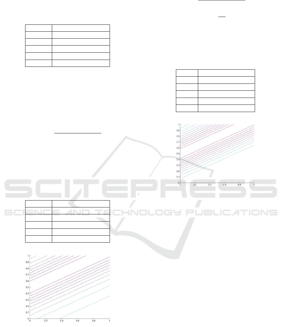
The error profile is shown in Table 3. The
numerical result has relatively small errors. The
contour plot is shown in Figure 2.
Table 3: Error profile for experiment 3.
Error in experiment 3
Figure 2: The contour plot for experiment 3.
3.3.4 Experiment 4
We borrow the same case as experiment 3, but
u
is as follow.
The error profile is shown in Table 4. The
numerical result has relatively small errors. The
contour plot is plotted in Figure 3.
Table 4: Error profile for experiment 4.
Error in experiment 4
Figure 3: The contour plot for experiment 4.
3.3.5 Experiment 5
In the experiment, we use
,
and
for the boundary data is
The streamline function used is where
Our experiment shows that boundary data has a
profound effect upon the method. Figure 4 shows
that the numerical solution is free from oscillation.
Figure 5 and 6 show the contour plot with
and
respectively. As can be studied, the
numerical solutions on smooth mesh produce a finer
approximation than numerical solutions on coarse
meshes.
The Least-Squares Finite Element and Minimum Residual Method for Linear Hyperbolic Problems
281
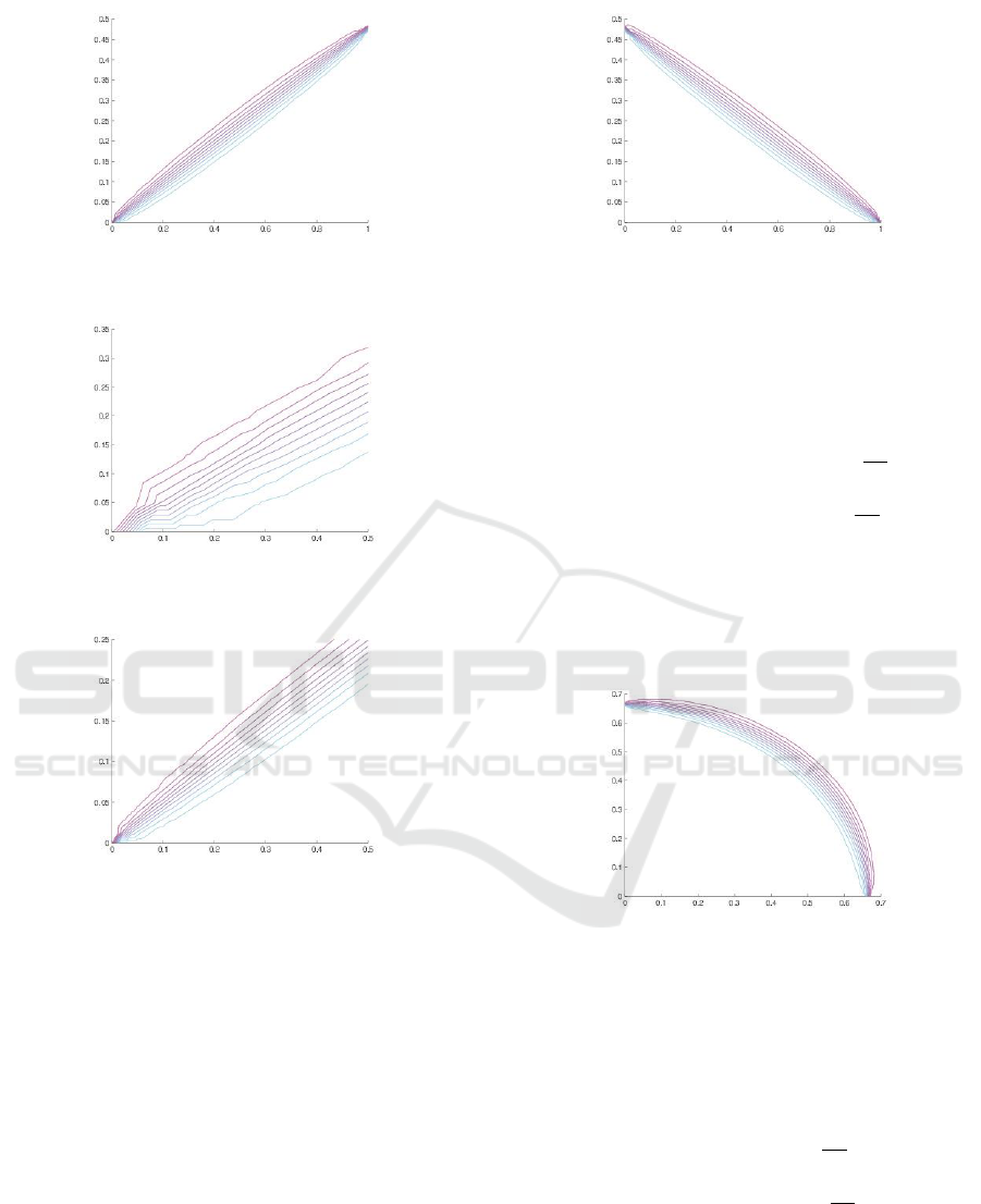
Figure 4: The contour plot for experiment 5.
Figure 5: The contour plot for
Figure 6: The contour plot for
3.3.6 Experiment 6
This experiment is the same as experiment 5, but
and
is given as
follow.
The streamline function used is The
contour plot is plotted in Figure 7. Again, our
solution is free from oscillation.
Figure 7: The contour plot for experiment 6.
3.3.7 Experiment 7
Here
and
for the
boundary data is
The contour plot is plotted in Figure 8. Figure 8
shows that the solution is free from oscillation.
Figure 8: The contour plot for experiment 7.
3.3.8 Experiment 8
In this experiment, we use
and
chosen is as follow.
The numerical solution for experiment 8 that
shown in Figure 9 shows that the solution is also
free from oscillation.
ICMIs 2018 - International Conference on Mathematics and Islam
282
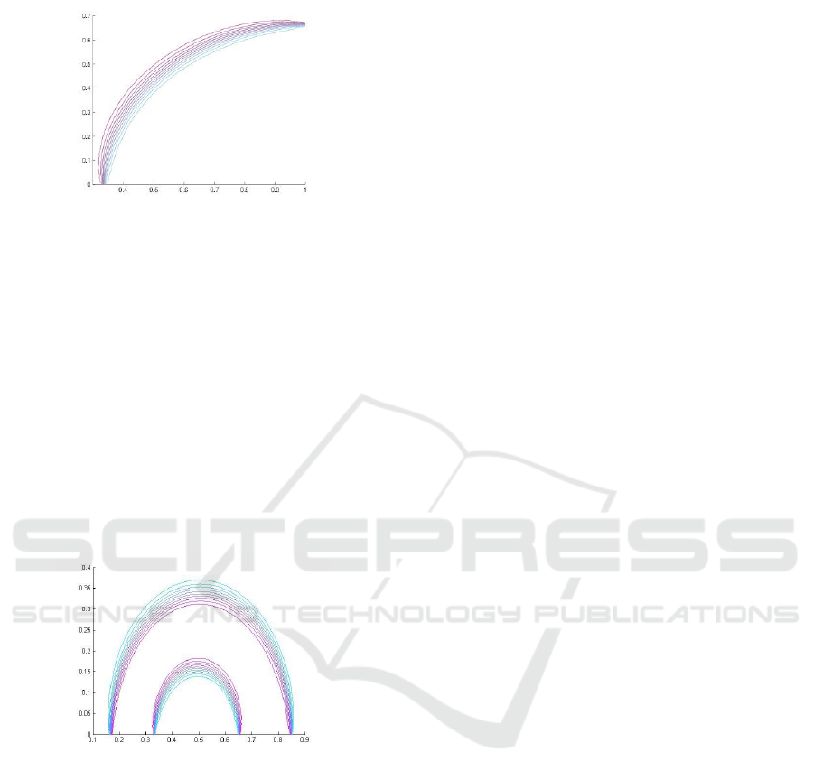
Figure 9: The contour plot for experiment 8.
3.3.9 Experiment 9
In the last experiment, we use
and
The contour plot for experiment 9 is plotted in
Figure 10. The conclusion obtained is the same
conclusion as the previous experiment.
Figure 10: The contour plot for experiment 9.
4 CONCLUSIONS
Based on the previous section, it can be concluded
that the least-squares finite element and minimum
residual method can efficiently solve the linear
hyperbolic equation without oscillation. The
numerical result shows that the numerical error is
relatively small for continuous problem. In addition,
the solution is free from oscillation for discontinuous
problem.
REFERENCES
Bochev, P. B., Choi, J., 2007. A Comparative Study of
Least-squares, SUPG and Galerkin Methods for
Convection Problems. International Journal of
Computational Fluid Dynamics Vol. 15. pp. 127-146,
Overseas Publishers Association.
Burman, E., 2010. Consistent SUPG-Method for Transient
Transport Problems: Stability and Convergence.
Computer Methods in Applied Mechanics and
Engineering Vol.119, pp. 1114-1123. Elsevier.
De, H. S., Manteuffel, T. A., Mccormick, S.F., 2004.
Least-Squares Finite Element Methods and Algebraic.
SIAM J. SCI. COMPUTVol. 26. No. 1. pp. 31-54.
Society for Industrial and Applied Mathematics.
Elman, H., Silvester, D., Wathen, A., 2005. Finite
Elements and Fast Iterative Solvers: with Application
in Incompressible Fluid Dynamics, Oxford University
Press, New York.
Mu, L., Ye, X., 2017. A Simple Finite Element Method
for Linear Hyperbolic Problems. Journal of
Computational and Applied Mathematics Vol.330, pp.
330-339. Elsevier.
Olson, L., 2004. A Dual Least-Squares Finite Element
Method for Linear Hyperbolic PDEs: A Numerical
Study. Department of Applied Mathematics.
Reed, W. H., Hill, T. R., 1973. Triangular Mesh Methods
for the Neutron Transport Equation. Technical Report
LA-UR-73-479. Los Alomos Scientific Laboratory.
Yu-Ling Lai, Wen-Wei Lin, Pierce, D., 1997. Conjugate
gradient and minimal residual methods for solving
symmetric indefinite systems. Journal of
Computational and Applied MathematicsVol. 84. pp.
243-256, Elsevier.
The Least-Squares Finite Element and Minimum Residual Method for Linear Hyperbolic Problems
283
