
Geographically Weighted Regression Model for Corn Production in
Java Island
Yuliana Susanti, Hasih Pratiwi, Respatiwulan, Sri Sulistijowati Handajani and Etik Zukhronah
Study Program of Statistics, Universitas Sebelas Maret, Ir. Sutami 36A Kentingan, Surakarta, Indonesia
Keywords: Geographically Weighted Regression, Corn, Java.
Abstract: In Java Island, corn is the second food commodity after rice. The need for corn increases every year, but it
does not match which the amount of corn production for the respective year. Factors that cause corn
production in Java are harvested area, rainfall, temperature, and altitude. The main problem faced in
increasing corn production still relies on certain areas, namely Java Island, as the main producer of corn.
Differences in production are what often causes the needs of corn in various regions cannot be fulfilled and
there is a difference in the price of corn. To fulfill the needs of corn in Java, mapping areas of corn
production need to be made so that areas with potential for producing corn can be developed while areas
with insufficient quantities of corn production may be given special attention. Due to differences in
production in some areas of Java which depend on soil conditions, altitude, rainfall, and temperatures, a
model of corn production will be developed using the Geographically weighted regression (GWR) model.
Based on the GWR model for each regency/city in Java Island, it can be concluded that the largest corn
production coming from Rembang regency.
1 INTRODUCTION
Java Island is one of the islands in Indonesia, most
of which are widely used for the agriculture sector.
Java Island has a fertile soil, surrounded by
volcanoes making it suitable for agricultural areas.
The potential of agriculture in Java is spread evenly
throughout the region which includes rice, corn, and
crops. Corn is a second food commodity after rice,
but it is also used for animal feed and industrial raw
materials.
Corn production in Java is influenced by several
factors, including harvested area, rainfall,
temperature, and altitude. According to Purwono
and Hartono [1], sufficient air temperature for
optimal growth of corn is between 23 ° C to 27 ° C,
while rainfall is ideal for corn crops between 100
mm to 250 mm per month. In addition, different
altitude areas also affect the amount of corn
production. According to Effendi and Sulistiati
(1991), optimal corn production is produced at an
altitude between 100 meters and 600 meters above
sea level.
The Geographically Weighted Regression
(GWR) model is the development of a regression
model where each parameter is calculated at each
observation location, so that each observation
location has different regression parameter values.
The response variable y in the GWR model is
predicted by a predictor variable in which each
regression coefficient depends on the location where
the data is observed. In Susanti et al. [3], obtained
result that the data on corn in Java has spatial effects
both lag and error, but has low R
2
value. Therefore,
the purpose of this research is to model with point
approach method that is GWR model by using a
model of the best regression model for corn
production data in Java Island 2015.
2 LITERATURE REVIEW
2.1 Linear Regression Model
A linear regression model is a relationship model
between an independent variable (x) and a dependent
variable (y). The linear regression model with p
independent variables given as follow:
p
k
iikki
xy
1
0
(1)
where i = 1, 2, ... , n.
Susanti, Y., Pratiwi, H., Respatiwulan, ., Handajani, S. and Zukhronah, E.
Geographically Weighted Regression Model for Corn Production in Java Island.
DOI: 10.5220/0008518201310135
In Proceedings of the International Conference on Mathematics and Islam (ICMIs 2018), pages 131-135
ISBN: 978-989-758-407-7
Copyright
c
2020 by SCITEPRESS – Science and Technology Publications, Lda. All rights reserved
131

1
2
n
ε
The matrix form of the equation (1) is
y = Xβ + ε
where
1
2
n
y
y
y
y
,
11 12 1
21 22 2
12
1
1
1
p
p
n n np
x x x
x x x
x x x
X
,
0
1
p
β
,
.
The parameter estimation is
ˆ
TT
1
β X X X y
with
ˆ
β
is
an unbiased estimator for β. The estimated value for
y and ε are
ˆ
ˆ
yXβ
and
ˆ
ˆˆ
ε y y y Xβ
. The
testing statistic F of regression model is
, where H
0
is reject if
, and partial parameter test of regression
model is
where H
0
is rejected if
or
.
2.2 GWR Model
The GWR model can be written as follows
(Fotheringham et. al, 2002).
0
1
,,
p
i i i k i i ik i
k
y u v u v x
, (2)
where y
i
: the value of observation of the dependent
variable for the i
th
location, (u
i
,v
i
): the coordinate
point (longitude, latitude) from the i
th
location of the
observation, β
k
(u
i
,v
i
): the regression coefficient of
the k
th
independent variable on the i
th
location of
observation, x
ik
: the observation value of the
independent variable on the i
th
location, and ε
i
: the
observed i
th
error, which is assumed to be identical,
independent and normally distributed with zero
mean and constant variant.
2.3 Estimation of Parameter GWR
Model
Each parameter from the GWR model is calculated
at each observation location, so each location has
different regression parameters. The estimation of
parameters with weighted least square (WLS) of the
GWR model is derived from equation (2), the result
is
1
ˆ
, , ,
TT
i i i i i i
u v u v u v
β X W X X W y
(3)
where W(u
i
,v
i
) = diag(w
1
(u
i
,v
i
),… ,w
n
(u
i
,v
i
)).
The estimator of
ˆ
,
ii
uvβ
equation (3) is an unbiased
and consistent estimator for
,
ii
uvβ
(Nurdim,
2008).
So, the prediction value of y at the observation
location can be obtained by:
1
ˆ
ˆ
, , ,
T T T T
i i i i i i i i i
y u v u v u v
x β x X W X X W y
.
The estimator of
ˆ
,
ii
uvβ
from equation (3) is an
unbiased and consistent estimator for
,
ii
uvβ
(Nurdim 2008).
2.4 The Weighting of the GWR Model
The kernel function is one of the weighting methods
of the GWR model that can be used to determine the
weighting for each different location if the distance
function (w
j
) is a continuous and monotonous
function (Chasco, Garcia, and Vicens, 2007).
Weights that are formed by using this kernel
function are the Gaussian distance function,
Exponential function, Bisquare function, and
Tricube kernel function (Lesage, 1997). In this
research we use the weighted functions Gaussian as
follow:
,
j i i ij
w u v d h
,
where is the normal standard density and σ
denotes the standard deviation of the distance vector
by d
ij
is
22
jijiij
vvuud
the distance of
Euclidean between location (u
i
,v
i
) to location (u
j
,v
j
)
and h usually called the smoothing parameter
(bandwidth) and the weighted function bisquare:
The method is used to select the optimum
bandwidth, one of which is the method of Cross
Validation (CV) which is defined as follows:
2
1
ˆ
()
n
ii
i
CV h y y h
,
where
hy
i
is the estimator value of the
observations y
i
at the site (u
i
,v
i
) are omitted from the
estimation process. To obtain an optimal h value, it h
is chosen from the minimum CV value.
ICMIs 2018 - International Conference on Mathematics and Islam
132

2.5 Hypothesis Testing of the GWR
Model
The form of hypothesis testing the significance of
partial parameters GWR model is as follows
0
H : , 0
k i i
uv
1
H:
0,
iik
vu
where k = 1, 2, … ,p.
The partial test statistic of the GWR model is
If the selected level of significance is equal α, then
the decision taken under H
0
is rejected H
0
or in other
words a significant parameter to the model if
(Nugroho, 2018).
2.6 Spatial Heterogeneity Test
According to Anselin (1988), by using Breusch-
Pagan (BP) test method to test the spatial
heterogeneity, the hypothesis is
H
0
:
2 2 2 2
12 n
H
1
: at least one
22
i
The value of BP test is
1
1/ 2
T T T
BP
f Z Z Z Z f
~ X
2
(p)
,
where:
ˆ
i i i
e y y
12
, , ,
T
n
f f ff
where
2
2
1
i
i
e
f
and Z is the matrix .
H
0
is rejected if
2
p
BP
or if p-value < α.
We use the Akaike Information Criterion (AIC) or
determination coefficient to select the best model.
The AIC is defined as follows:
AIC = D(h) + 2K(h)
where
n
i
h
i
v
i
u
i
y
i
y
i
yh
i
v
i
u
i
y
i
yhD
1
,,
ˆ
/,,
ˆ
ln ββ
D(h) represents the value of deviants model with
bandwidth (h) and K represents the number of
parameters in the model with bandwidth (h). The
model with the minimum AIC value or with the
largest local coefficient of determination R
i
2
is the
best model, where
3 RESEARCH METHOD
We used data of corn production in Java Island on
2015 from Badan Pusat Statistik (BPS, 2016): corn
production as the dependent variable and area of
corn harvest, temperature, rainfall, and altitude of
each regency/city as the independent variables. The
first step is to construct the GWR model by choosing
the best bandwidth. After that, there will be
estimated the parameter and determined the local
coefficient of determination, so it can produce the
model for each observation point. Next, testing the
GWR model hypothesis, selected the best model
with AIC or R
2
, and interpret the results.
4 RESULT AND DISCUSSION
Linear regression model of corn production in
Indonesia in 2015, by using ordinary least square
(OLS) method, can be written by
(4)
In linear regression model (4), there is one
variable that significantly affected i.e. harvested
area. The linear regression model can be written as
follows
(
it means that 39.4 % corn production
in Java Island in 2015 could be explained by the
corn harvested area. Meanwhile, the rest at 60.6 %
was explained by other unobserved factors. The
values of parameter estimation and p-value to one
parameter could be observed in Table1.
Table 1: The parameter estimation value and p value.
Independent
variable
Parameter
estimation
P value
Constant
613425
0.03978*
Harvested
area
0.143016
0.00000*
( 1)np
Geographically Weighted Regression Model for Corn Production in Java Island
133
As see in Table 1, the regression model (5) has a
significant influence because of p-value < 0.05.
Then, regression assumption model testing was done
with the result showing that an unfulfilled of
homogeneity assumptions. This can be seen from the
BP value = 16.2699>
= 3.84. (with prob. =
0.00005). So that it can be concluded that there is
heteroscedasticity in several districts/cities observed.
Because the assumption of variance homogeneity is
not fulfilled, it is solved by GWR analysis.
The first step in the GWR modeling is to
determine the bandwidth values of the Gaussian
kernel and bisquare weighting functions
Table 2 shows the bandwidth values with the
Gaussian and bisquare kernel weighted function:
Table 2: The bandwidth values and minimum AICc.
Bandwidth
Minimum AICc
Gaussian
79.533
2355.154
Bisquare
39.000
2354.138
From Table 2, it is found that the best weighing
bandwidth is 39. The weighing function, used in
processing, is bisquare with longitude and latitude
for each observation point with lots of 103 points of
observation data. The processing of corn data
modeled using the GWR model will produce 103
GWR models for each regency/city. The resulting
GWR model will be different for each region and
significant variables will also be different for each
regency/city. Table 3 show 5 models with the
highest R
2
for corn production.
Table 3: GWR Model for Corn production in Java Island
Regen
cy/
Cities
Regression
Model
t
Local
R
2
β
0
β
1
Blora
=180.407+0.16
3X
1
180.407*
0.163
0.941
Rembang
=255.664+0.16
8X
1
255.664*
0.168
0.947
Ponorogo
=499+0.153X
1
499*
0.153
0.922
Nganjuk
=385.44+0.156
X
1
385.44*
0.156
0.927
Bojone-
goro
=445.50+0.163X
1
445.50*
0.163
0.937
*Not significant to t
(0.025,101)
= 1.984
From Table 3, there are the five best models that
have the highest determination coefficient. For
example, we take model for the regency of Rembang
and we obtain the determinan coefficient R
2
= 0,941.
= 255.664+0.168X
1
(6)
The model has a coefficient of determination of
0.947. It means that 94.7% of production can be
explained by a harvested area while the other 5.3%
can be explained by other variables. In addition,
local values of R
2
close to 1 indicate that the model
is good. Then test the model parameters, as follows:
i. H
0
:β
1
(u
1
,v
1
) = 0
H
1
:β
1
(u
1
,v
1
) ≠ 0
ii. Critical Area: Null is rejected if
|t|>t
((0.025,101))
=1.984
iii. Statistical test: |t|=6.373
iv. Because of t = 6.373 > t
(0.025, 101)
= 1.984
then H
0
rejected which means that equation
(6) is significant.
From the GWR model obtained, then made
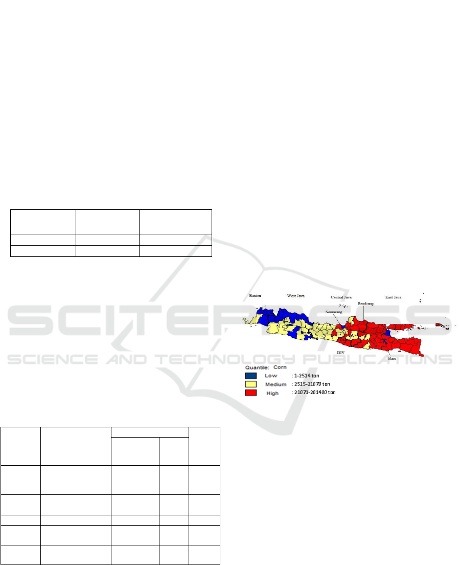
predictions on corn production as in Figure 1. Figure
1 shows classification of corn production in Java
Island. The difference of color indicates high,
medium and low corn production. Comparison of
high, medium and low corn productions were
35.9 %, 33.9%, and 30.2% respectively.
Figure 1: The Classification of all Region in Java Island.
5 CONCLUSIONS
Based on GWR model for each regency/city, the
largest corn production is coming from Rembang
regency with R
2
is 94.7%, which means that 94.7%
of production can be explained by harvested area
while the other 5.3% can be explained by other
variables.
ACKNOWLEDGMENTS
The author would like to thank the Indonesian
Ministry of Research, Technology and Higher
Education as well as Universitas Sebelas Maret for
ICMIs 2018 - International Conference on Mathematics and Islam
134

financial support through Grant of Leading Research
of University 2018.
REFERENCES
Anselin, L., 1988. Spatial Regression Analysis in R.
University of Illinois, Urbana.
Badan Pusat Statistik, 2016. Indonesia Dalam Angka
2016. Jakarta.
Chasco, C., Garcia, I. and Vicens, J., 2007. Modeling
Spatial Variations in Household Disposable income
with Geographically Weighted Regression. Munich
Personal RePEc Archive, Paper No.1682.
Effendi, S. and Sulistiati, N., 1991. Bercocok Tanam
Jagung. Yasagna, Jakarta.
Fotheringham, A. S., Brunsdon, C., and Charlton, M. E.,
2002. Geographically Weighted Regression: The
Analysis of Spatially Varying Relationships. Wiley,
Chichester.
Lesage, J. P., 1997. Regression Analysis of Spatial Data.
Journal Regional and Polic Vol. 27, No. 2, pp. 83-84.
Nurdim, F. I., 2008. Estimasi dan Pengujian Hipotesis
Geographically Weighted Regression (Studi Kasus
Produktivitas Padi Sawah di Jawa Timur). Thesis,
Jurusan Statistika FMIPA ITS, Surabaya.
Nugroho, I. S., 2018. Geographically Weighted
Regression Model with Kernel Bisquare and Tricube
Weighted Function on Poverty Percentage Data in
Central Java Province. IOP Conf. Series: Journal of
Physics, Series 1025(2018)012099.
Purwono and R. Hartono, 2011. Bertanam Jagung
Unggul. CV Penebar Jakarta.
Susanti, Y., Pratiwi, H., Respatiwulan, Handajani, S.S.
and Zukhronah, E., 2018. The Prediction model of
corn availability in Java Island using spatial
regression. International Conference on Science and
Applied Science, Surakarta.
Geographically Weighted Regression Model for Corn Production in Java Island
135
