
Ordinary Kriging Method using Isotropic Semivariogram Model for
Estimating the Earthquake Strength in Bengkulu Province
Fachri Faisal
1
, Pepi Novianti
2
and Siska Yosmar
1
1
Department of Mathematics, Bengkulu University, Bengkulu, Indonesia
2
Department of Statistics, Bengkulu University, Bengkulu, Indonesia
Keywords: Ordinary Kriging, Semivariogram, Isotropic, Earthquake.
Abstract: Ordinary kriging method is a method that gives the best unbiased estimator. Kriging method has been applied
to several earthquake studies. Faisal (2014) uses isotropic semivariogram models using the linear program
method in the earthquake event data sample in Bengkulu. However, the kriging method has not been used to
estimate the earthquake strength. This study aims to apply the ordinary kriging method to estimate the
strengths of the earthquake in Bengkulu Province and its surrounding areas. The semivariogram model used
in the parameter estimation is an isotropic semivariogram model. We use data earthquake events in the range
from 99.00°E to 104.00°E on the latitude position and from 6.00°S to 2.00°S on the longitude position. The
result shows that the semivariogram model that can be used is the spherical model with Sill = 0.1907015 and
Range = 0.07929616 and the exponential model with Sill = 0.1898991 and Range = 0.01622501. The
maximum earthquake strength estimation on the spherical model is Mw 7.5249 and the maximum on the
exponential model is Mw 7.5254. These models show that the epicenter of the greatest earthquake estimation
is on 102.0833°E, 4.7045°S.
1 INTRODUCTION
Spatial data is data that contain information about
location attributes and information. Spatial data are
presented in the geographical position of objects,
locations, shapes, and relationships with other
objects. Analysis of spatial data requires more
attention than analysis of non-spatial data. Spatial
analysis is an analysis that considers location
attributes, as well as absolute locations (coordinates).
One of the sciences that use spatial analysis is
geostatistics.
Geostatistics emerged in the early 1980s as a
combination of mining science, geology,
mathematics, and statistics. Geostatistics was
originally developed in the mineral industry to assess
the mineral reserves in the earth. Geostatistics
recognizes spatial variations on the large and small
scale, or the spatial trends and the spatial correlation.
Geostatistics is used to predict data at locations that
have not been measured (Fischer & Getis, 2010)
One of the basic tools in geostatistics is a
semivariogram that explains the variability of data at
certain distances and directions. Semivariogram is a
real function to show the spatial correlation measured
at the sample location. Semivariogram is presented as
a graph that shows the variance in measuring the
distance between all pairs of sample locations. There
are two types of semivariogram namely isotropic
semivariogram and anisotropic semivariogram. The
semivariogram used in the kriging procedure to
interpolate unobserved locations.
Kriging is a geostatistics method that utilizes a
semivariogram model to estimate values in other
regions that have not been sampled (Rubeis et al.,
2005). There are different types of Kriging
techniques, such as Ordinary Kriging, Universal
Kriging, Indicator Kriging, Co-kriging, and others.
The choice of which kriging to use depends on the
characteristics of the data (Mesić Kiš, 2015).
Ordinary kriging is the most widely used kriging
method. It serves to estimate a value at a point of a
region for which a variogram is known, using data in
the neighborhood of the estimation location
(Wackernagel, 2003).
Along with the development of science and
technology, geostatistics continues to grow, and its
application extends to various fields, such as weather,
climate, disaster, and population. In the field of
disaster, several earthquake studies using the Kriging
34
Faisal, F., Novianti, P. and Yosmar, S.
Ordinary Kriging Method using Isotropic Semivariogram Model for Estimating the Earthquake Strength in Bengkulu Province.
DOI: 10.5220/0008516800340040
In Proceedings of the International Conference on Mathematics and Islam (ICMIs 2018), pages 34-40
ISBN: 978-989-758-407-7
Copyright
c
2020 by SCITEPRESS – Science and Technology Publications, Lda. All rights reserved

method have been carried out before. Research
conducted by Carr et.al (1986) applied disjunctive
kriging to estimate ground movements in the event of
an earthquake. Furthermore, Carr et al. (1989)
continued his research by comparing universal
kriging and ordinary kriging method to estimate the
ground motion in the event of an earthquake. Sugai et
al. (2015) introduced a practical method to estimate
the specific distribution of ground motion earthquake
events based on ordinary kriging analysis. Recent
research on the application of ordinary kriging was
carried out by Bekti et al. (2017) on the peak ground
acceleration (PGA) data in Banda Aceh in 2006 and
the results are Ordinary Kriging can be applied to
predict PGA.
The kriging method is considered as the best
estimation method in terms of the accuracy of its
assessment. The ordinary kriging method is a method
of estimating a random variable at a certain point
(location) by observing similar data in another
location with the mean data assumed to be constant
but unknown in value. This method is a method that
provides the best linear unbiased estimator (BLUE).
Hence, the ordinary kriging method can be used in
earthquake events. The other hand, in reality, the
population average of earthquake events is difficult to
be known.
Bengkulu Province is one of the provinces located
at the meeting of the Indo-Australia and Eurasia
tectonic plates which are the main generators of high
earthquake activity. The movements caused by these
two plates can cause active faults which are
generators of seismicity in parts of Sumatra.
Bengkulu is also among two active faults, the
Semangko and Mentawai faults. This condition
makes Bengkulu Province the most vulnerable to
earthquake disasters (Hadi et al., 2010).
Faisal (2014) compared Matheron (classic) and
Cressie-Hawkins (robust) isotropic semivariogram
models using the linear program method in the
earthquake event data sample in the coastal area of
Bengkulu. From the results of the case study, the
Spherical theoretical semivariogram model was the
best semivariogram model obtained from the results
of the Matheron isotropic experimental
semivariogram. However, in this study, the kriging
method has not been used to estimate earthquake
strength in Bengkulu area
Based on the previous research, we interested in
conducting further research. The purpose of this study
was to predict the strength of earthquakes in
Bengkulu Province and its surrounding areas based
on the epicenter of an earthquake that occurred in
some years. We use the ordinary kriging with the
isotropic semivariogram model. The final objective is
a mapping of the predicted strength of the earthquake
from the selected model. To facilitate the calculation
of the kriging and mapping, we use R software.
2 LITERATURE REVIEW
2.1 Semivariogram Analysis
Variogram is a tool in geostatistics that is used to
describe spatial correlations of data. In Plotting of
variogram, the low value will be close to other low
costs and large value will be near other large values.
The values can be visualized in a variogram graph as
a function of distance. Variogram determines the
distance where the values of the observation data are
independent or have no correlation. The symbol of the
variogram is 2γ, while semivariogram is half of the
variogram with the symbol γ. This semivariogram is
used to measure spatial correlation ( Wackernagel,
2003).
The experimental variogram is a variogram
calculated from the observed data. Variogram is
formulated as follows:
(1)
assume that the data are second order stationary,
equation (1) can be written as follows:
(2)
Since semivariogram is half of the variogram, then
from equation (2) can be written:
, (3)
where γ(h) is a semivariogram. The above
semivariogram is also called theoretical
semivariogram. There are two types of
semivariogram: isotropic semivariogram (γ(h)
depends only on distance h) and anisotropic
semivariogram (γ (h) depends on distance h and
direction).
A semivariogram is a statistical tool for
describing, modeling and explaining spatial
correlations between observations. An experimental
semivariogram is a semivariogram obtained from
known data. The estimator of semivariogram
proposed by Matheron (1962) in Cressie (1993) is:
Ordinary Kriging Method using Isotropic Semivariogram Model for Estimating the Earthquake Strength in Bengkulu Province
35
( )
( )
=
−+=
)(
1
2
)()(
2
1
ˆ
hN
i
ii
szhsz
hN
h
(4)
where s
i
is location of sample (coordinate), Z(
i
s
)
data value in location
i
s
and |N(h)|: pairs (
i
s
,
i
s
+h)
with distance h .
Semivariogram has properties s follows:
1. Semivariogram value at the origin is zero:
.
2. Semivariogram values are always non-negative:
3. Semivariogram is an even function:
.
The semivariogram plot of distance h gives an
experimental semivariogram plot. Experimental
semivariograms obtained from data usually have
irregular shapes that are difficult to interpret and
cannot be directly used in assessments. These
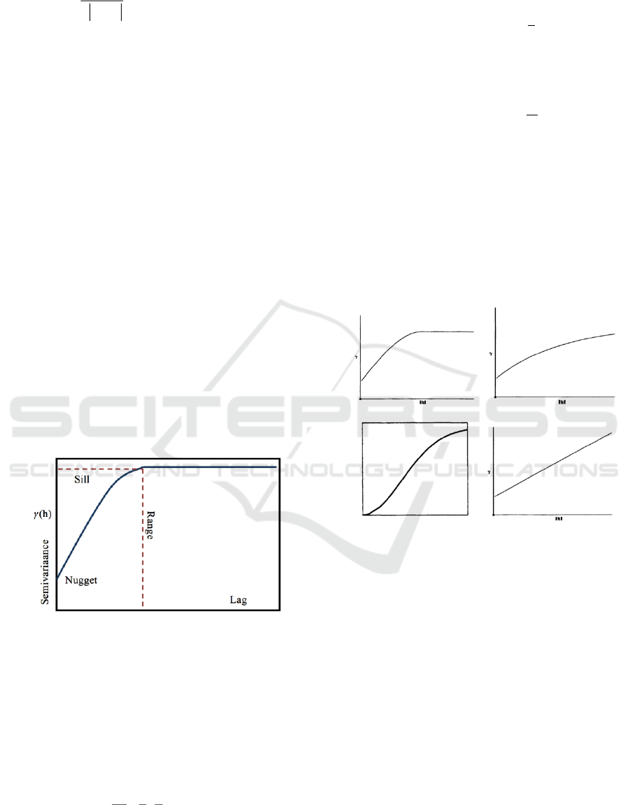
parameters are:
a. Range is the maximum distance where there is
still a correlation between data.
b. Sill is a semivariogram value that does not
change for unlimited h. The sill value generally
approaches the data variance.
c. The Nugget effect is a discontinuous
phenomenon around the starting point.
Figure 1: Component of semivariogram graph.
In the semivariogram prediction, the theoretical
semivariogram model is fitted in the experimental
semivariogram
( )
h
ˆ
. There are four theoretical
semivariogram models are (Cressie, 1993; Amstrong,
1998):
1. Spherical model:
+
−+
=
ahCC
ah
a
h
a
h
CC
h
,
0,
2
1
2
3
)(
0
3
0
(5)
2. Exponential model:
(6)
3. Gaussian model:
(7)
where C
0
: nugget variance,
: sill, and a:
range
4. Linear Model
(8)
where α is a gradient.
(a) (b)
(c) (d)
Figure 2: The theoretical semivariogram models: (a)
Spherical Model, (b) Exponential Model, (c) Gaussian
Model and (d) Linear Model.
2.2 Ordinary Kriging
The ordinary kriging method is a method of
estimating a random variable at a certain point
(location) by observing similar data in another
location with the mean data assumed to be constant
but unknown in value. In the ordinary kriging
method, the known sample are used as linear
combinations to estimate the points around the
sample area (location). In other words, to estimate
any non-sampled point (
can use a linear
combination of random variables
and kriging
weight values respectively, mathematically can be
written with:
ICMIs 2018 - International Conference on Mathematics and Islam
36
, (8)
Where
is the estimated value of the random
variable at points
, and
is the value of the
random variable
at the i-point, and
is the
kriging weight at the i-point (Pfeiffer and Robinson,
2008). Whereas the variance of the estimated error
(kriging variance) can be expressed by:
(7)
where parameter m is the Lagrange multiplier.
3 METHODS
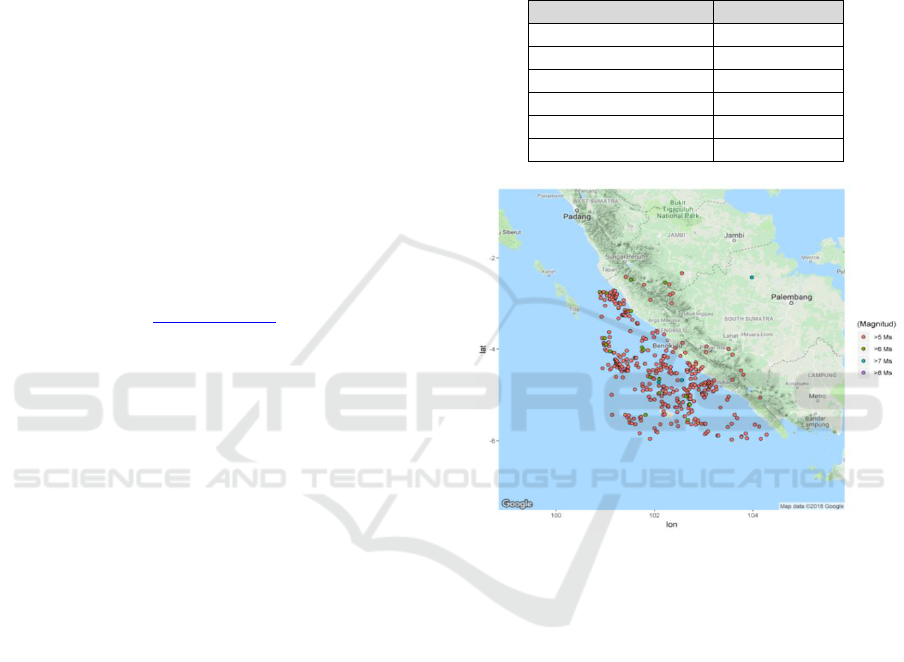
We use data of the earthquake events with
magnitudes above Mw 5.0 that occurred in Bengkulu
Province from 2000 to 2016. The 365 data obtained
from the website www.usgs.com. The variables of
data are the coordinate position of the center of the
earthquake, latitude, longitude, and magnitude. Based
on the longitude position, earthquake events in the
data range from 100.00°E to 105.00°E, while based
on the latitude position, the minimum data is at
6.00°S, and the maximum is at 2.00°S.
The steps of analysis in this study are:
1. Collect data of earthquake occurred in the
Bengkulu Province and its surrounding areas.
2. Perform descriptive statistics for magnitude
variable.
3. Calculate Experimental Semivariograms using
equation (4) and display a variogram graph.
4. They fit theoretical Semivariogram from
variogram graph, Spherical, Exponential,
Gaussian and Linear models.
5. Perform a model validation test to determine
whether the theoretical semivariogram model that
will be used in the kriging method is the best
model with the smallest remaining sum squares
(RSS) value compared to the other models.
6. Map a contour of earthquake strength estimation
in Bengkulu Province and the surrounding areas.
4 RESULTS AND DISCUSSION
The descriptive statistics of the data are shown in
table 1. shows that the minimum earthquake is Mw 5
and the maximum earthquake occurred with a
strength of Mw 8.4. This Mw 8.4 earthquake occurred
on December 9, 2007, with the epicenter of the
earthquake at 101.37°N and 4.44°S. The average
earthquake data used is Mw 5.33 with a standard
deviation of 0.417. The median earthquake strength is
Mw 5.2 and the range is Mw 3.4.
Table 1: Statistics of the earthquake strength in Bengkulu
Province.
Statistic
Magnitude
Mean
5.333
Standard Deviation
0.417
Median
5.200
Range
3.400
Maximum
8.400
Minimum
5.000
Figure 3: The distribution of earthquake events with
magnitudes above Mw 5 that occurred in Bengkulu
Province from 2000 to 2016.
Figure 3 describes that the central point of the
earthquake event in Bengkulu Province and its
partners occurred a lot in the sea and most of the
earthquakes were between Mw 5-6.
The results of the calculation and experimental
semivariogram images can be seen in Table 2 and
Figure 4. The experimental semivariogram plot in
figure 4 shows that the first class has a semivariogram
value of 0.1875, then slightly decreases and rises back
to the maximum semivariogram of 0.2208 at a
distance of 0.2773. The semivariogram value
fluctuates around 0.1800 and slightly decreases
towards a stable value of 1.6 with a value of 0.1639.
Ordinary Kriging Method using Isotropic Semivariogram Model for Estimating the Earthquake Strength in Bengkulu Province
37
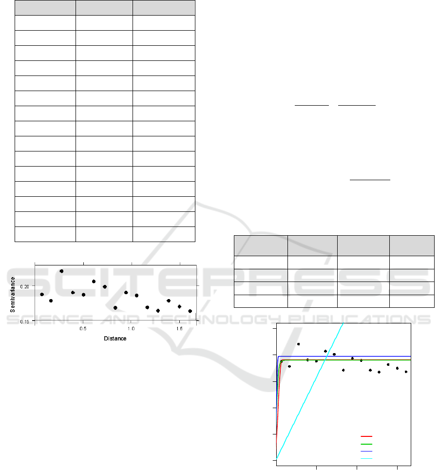
Table 2: Experimental semivariogram.
Number of pairs
Distance
Semivariogram
789
0.0709
0.1875
1564
0.1682
0.1786
1935
0.2773
0.2208
2280
0.3889
0.1903
2699
0.4990
0.1871
2966
0.6082
0.2061
3295
0.7201
0.1987
3676
0.8294
0.1685
3560
0.9401
0.1903
3656
1.0504
0.1857
3547
1.1595
0.1691
3473
1.2703
0.1644
3253
1.3815
0.1783
3251
1.4923
0.1699
3205
1.6018
0.1639
Figure 4: Experimental semivariogram graph.
Furthermore, the fitting of the theoretical
semivariogram model is conducted to determine the
value of the parameters and the model validation test
to determine the theoretical semivariogram model to
be used in the kriging method. The best model is
chosen based on the smallest value of Residual Sum
Squares (RSS). Parameters in the spherical,
exponential, Gaussian and linear models are shown in
Table 3 while fitting the experimental semivariogram
model with the theoretical model is shown in Figure
5.
The best semivariogram model is chosen based on
the sum square error value, where the smallest sum
square error value shows the best model. Based on the
sum square value error the spherical semivariogram
model shows the smallest number with a value of
39.68526. This number is slightly smaller than the
sum square error in the exponential model which is
worth 40.41875. Hence, this kriging estimation will
be used two models, namely spherical model with Sill
parameter = 0.1907015, Range = 0.07929616, and
Nugget = 0 and exponential model with Sill =
0.1898991, Range = 0.01622501, and Nugget = 0.
Following are the theoretical semivariogram models
used:
Spherical model:
Exponential model:
Table 3: Parameter of theoretical semivariogram model.
Variogram
Model
Sill
(Co+C)
Range (A)
Residual
SS
Spherical
0.1907015
0.07929616
39.68526
Exponential
0.1898991
0.01622501
40.41875
Gaussian
0.1968073
0.01198644
60.852
Linier
0.3135558
0
6463.833
Figure 5: Theoretical semivariogram model.
The central points that are estimated are in the
range from 100.00°E to 105.00°E, while based on the
latitude position, the minimum data is on 6.00°S, and
the maximum is on 2.00°S. The number of points to
be estimated is 10,000 points. Estimates are carried
0.5 1.0 1.5
0.00
0.05
0.10
0.15
0.20
0.25
Distance
Semivariance
Spherical
Exponential
Gaussia n
Linier
ICMIs 2018 - International Conference on Mathematics and Islam
38
out using the ordinary kriging at the determined
location to estimate the Z value. Here are the results
of estimating earthquake strength at points that are
not sampled using the spherical model:
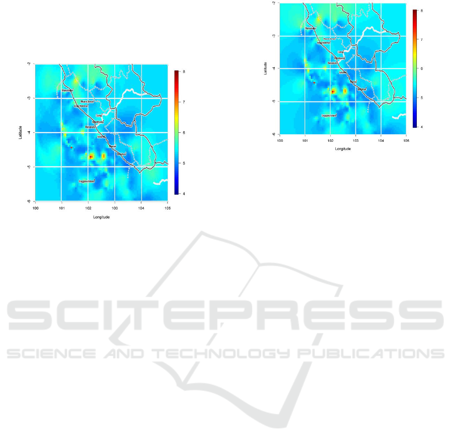
Figure 6: Contour map of the earthquake strength
estimation based on the spherical model.
Based on the earthquake strength contour map
above, the location of the dark blue is the location of
the epicenter of the earthquake with a power of Mw 4
– 5, while the light blue indicates the strength of Mw
5 – 6. From the color on the contour map on the
coordinates 100.00°E to 105.00°E and 6.00°S to
2.00°S, the potential for earthquakes with a strength
of Mw 4 – 6 is wider than that of an earthquake with
a magnitude of more than Mw 6. Besides that, there
are also areas with yellow and red colors. The yellow
color shows the area with an earthquake strength of
Mw 6 – 7 and the red color of the area with an
earthquake strength of Mw 7 – 8. The maximum
earthquake strength estimation on this contour map is
Mw 7.5249. The red areas are concentrated at several
points, which are around the points 101.3611°E,
4.4318°S and 102.0833°E, 4.7045°S, so that this area
is estimated to have earthquake strength above Mw 7.
In the area around 102.5833°E, 4.6590°S there is an
area with an orange color which shows the estimated
strength of the earthquake in the area around that
point is close to Mw 7.
Figure 7: Contour map of the earthquake strength
estimation based on the exponential model.
Figure 7 shows the estimated contour of
earthquake strength using the exponential model.
This contour shows the same pattern as the contour in
the spherical model, where light blue and dark blue
dominate the estimation area. The dark blue area is
the location of the epicenter of the earthquake with a
power of Mw 4-5, while the light blue indicates the
strength of Mw 5-6. The yellow color shows the area
with the earthquake strength of Mw 6 – 7 have lied
in the same area in the spherical model. The red color
is the area with the earthquake strength of Mw 7 – 8
are around the points 101.3611°E, 4.4318°S, and
102.0833°E, 4.7045°S. Maximum earthquake on the
exponential model predicted in the red area is Mw
7.5254.
5 CONCLUSIONS
From the results and discussion concluded that the
semivariogram model that can be used is a spherical
model with sill = 0.1907015 and range = 0.07929616
and an exponential model with sill = 0.1898991 and
range = 0.01622501. Based on the spherical model
and exponential model, the potential for earthquakes
with a strength of Mw 4 – 6 is wider than that of an
earthquake with a magnitude of more than Mw 6. The
maximum earthquake strength estimation on the
spherical model is Mw 7.5249 and maximum on the
exponential model is Mw 7.5254. Using both of
models, spherical and exponential model, it’s known
that the epicentre of the greatest earthquake
estimation is on 102.0833°E, 4.7045°S.
Ordinary Kriging Method using Isotropic Semivariogram Model for Estimating the Earthquake Strength in Bengkulu Province
39

ACKNOWLEDGMENTS
Research Projects Penelitian Produk Terapan
supported this work, Ministry of Research,
Technology, and Higher Education of Republic
Indonesia.
REFERENCES
Amstrong, M., 1998. Basic Linear Geostatistics. Springer-
Verlag Berlin Heidelberg, Germany.
Bekti R. D., Irwansyah, E., Kanigoro, B. and Theodorick,
2017. Ordinary Kriging and Spatial Autocorrelation
Identification to Predict Peak Ground Acceleration in
Banda Aceh City, Indonesia. Advances in Intelligent
Systems and Computing 662, pp. 318–325, September,
DOI: 10.1007/978-3-319-67621-0_29.
Carr, J. R.,FDeng, E. D., and Glass, C. E., 1986. An
Application of Disjunctive Kriging for Earthquake
Ground Motion Estimation. Mathematical Geology,
18(2): 197-213.
Carr, J. R., and Roberts, K. P., 1989. Application of
universal kriging for estimation of earthquake ground
motion: Statistical significance of results.
Mathematical Geology, 21(2): 255-265.
Cressie, N. A. C., 1993. Statistics for spatial data. John
Willey & Sons Inc, USA.
De Rubeis, V., Tosi, P., Calvino, G. And Solipaca, A.,
2005. Application of kriging technique to seismic
intensity data. Bulletin of the Seismological Society of
America, Vol. 95, No. 2, pp. 540–548.
Faisal, F., 2014. Aplikasi program linier dalam menentukan
nilai parameter model semivariogram teoritis.
Prosiding Semirata IPB Bogor.
Fischer, M. M. and Getis, A., 2010. Handbook of applied
spatial analysis: software tools, methods and
applications. Springer-Verlag Berlin Heidelberg, PP.
21.
Hadi, A. I., Suhendra and Efriyadi, 2010. Studi analisis
parameter gempa Bengkulu berdasarkan data single-
station dan multi-station serta pola sebarannya. Berkala
Fisika . Vol. 13 No. 4: 105-112.
Mesić Kiš, I., 2016. Comparison of Ordinary and Universal
Kriging interpolation techniques on a depth variable (a
case of linear spatial trend), case study of the Šandrovac
Field. The Mining – Geology - Petroleum Engineering
Bulletin, pp. 41–58.
Sugai, M., Mori, Y., and Ogawa, K., 2015. Application of
Kriging Method Into Practical Estimations Of
Earthquake Ground Motion Hazards. J. Struct. Constr.
Eng., AIJ, 80(707): 39-46.
Wackernagel, H., 2003. Multivariate Geostatistics, 3rd ed.
Springer, Berlin, Heidelberg.
ICMIs 2018 - International Conference on Mathematics and Islam
40
