
Detection of Heat Conduction Disturbance in
Cylindrical-Shaped Metal Chip using Kalman Filter and
Ensemble Kalman Filter
Nina Fitriyati, Gina Isma Kusuma and Irma Fauziah
Mathematics Study Program, Faculty of Sciences and Technology
UIN Syarif Hidayatullah Jakarta, Jl. Ir. H. Juanda No. 95 Ciputat, Banten, Indonesia
Keywords: Kalman Filter, Ensemble Kalman Filter, Heat Conduction, Diffusion Equation.
Abstract: The heat transfer process will be disrupted when a leak occurs. Therefore, we need a method that can be
used to detect the leak. In this paper, the leak detection in cylindrical-shaped metal chip simulated by give
the heat disturbances in some positions. We discuss the estimation of heat disturbance position using the
Kalman filter (KF) and the Ensemble Kalman Filter (EnKF) method where the state-space equation is
constructed by discretization of the diffusion equation using Forward-Time Central Space Method. We
divide the radius of this metal chip into 17 grids and simulate the detection of 1–4 disturbances in different
positions. The simulation result shows that the KF and EnKF method succeed to detect the disturbances.
However, the EnKF is more accurate than KF. The heat disturbances can be detected more clearly if the
temperature of disturbance is large enough, especially for detection in the edge of chip (close to inner radius
and outer radius). In addition, the detection of disturbances location is also affected by the number of grids.
The more number of grids, the more accurate the position of detection.
1 INTRODUCTION
Heat transfer is the process of transferring heat from
objects that have high temperatures to the objects
with lower temperatures. The flow of heat is all-
pervasive. There are three modes of heat transfer i.e.
conduction, convection, and radiation. Conduction is
one process of heat transfer from one solid to
another one that has a different temperature. Heat
convection is transfer of heat in fluid or gases, and
thermal radiation occurs in a range of
electromagnetic of energy emission (Lienhard,
1930).
One obstacle that can cause resistance to heat
conduction is the leakage of the conductor media.
Mathematically, several methods have been
developed to detect leaks in metals including the
Kalman filter and its development methods: adaptive
particle filter (Liu et al., 2005), Extended Kalman
filter (Emara-Shabaik et al., 2002), and EnKF
(Apriliani, 2011).
Inspired by Apriliani (2011), in this study, we
will detect the heat disturbances and its location in
the cylindrical-shaped metal chip using the Kalman
filter method and EnKF. The state-space equation
will be formed by the result of discretization of the
diffusion equation using Forward-Time Central
Space (FTCS) Method.
2 METHODOLOGY
According to Carslaw and Jeager (1959), the three
dimensional of heat equation in cylindrical
coordinates can be expressed by:
, (1)
where v is temperature, t is time, r is radius and k is
conductivity. If we heat the cylindrical with the axis
coincides with the z axis, the initial and boundary
conditions are independent of the coordinates of θ
and z.
The steady-state is a condition when several
process variables such as pressure, temperature,
location or position do not change with time. With
this steady-state, a process will be more easily
Fitriyati, N., Kusuma, G. and Fauziah, I.
Detection of Heat Conduction Disturbance in Cylindrical-Shaped Metal Chip using Kalman Filter and Ensemble Kalman Filter.
DOI: 10.5220/0008516400090014
In Proceedings of the International Conference on Mathematics and Islam (ICMIs 2018), pages 9-14
ISBN: 978-989-758-407-7
Copyright
c
2020 by SCITEPRESS – Science and Technology Publications, Lda. All rights reser ved
9

managed and planned. One-dimensional heat
conduction in a steady-state condition based on
Equation (1) is
(2)
The solution for equation (2) with the initial
conditions and boundaries:
,
and
is
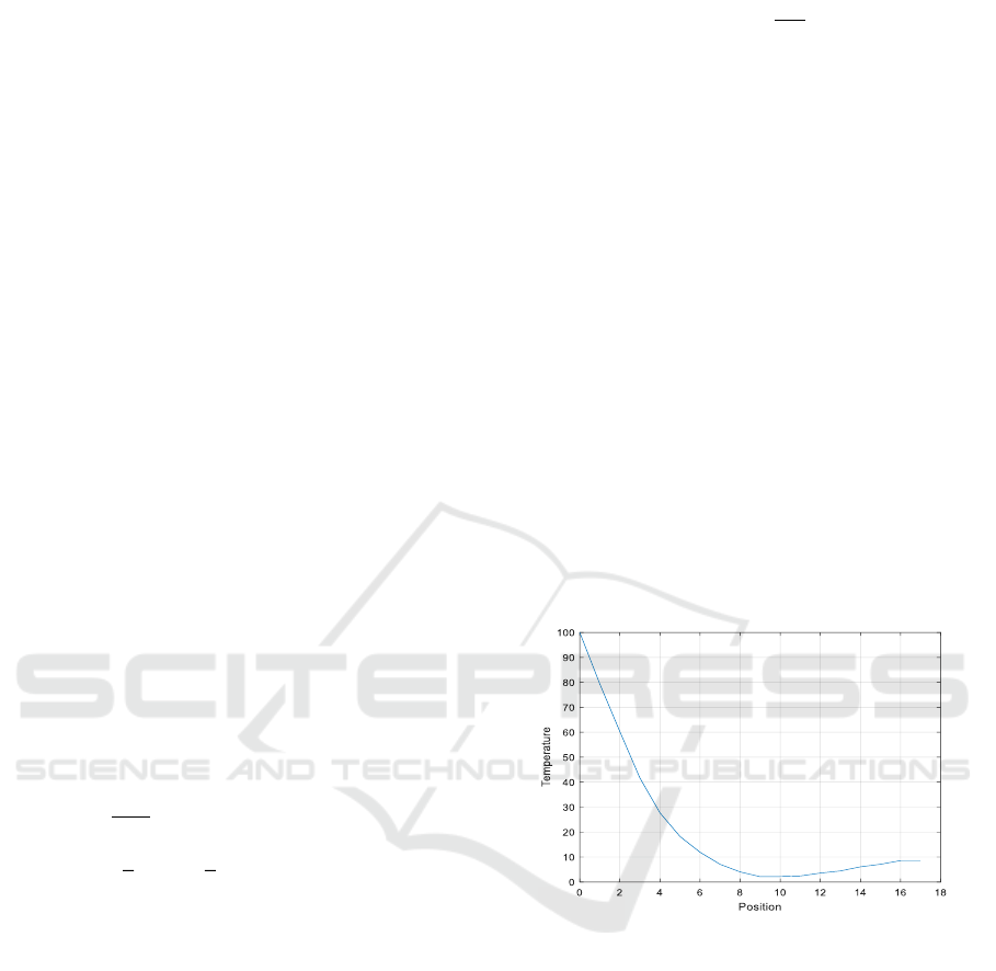
(3)
where is temperature. This heat transfer can be
illustrated in figure 1 and this object called
cylindrical-shaped metal chip.
Figure 1: The heat transfer in the cylindrical metal chip.
The FTCS discretization for Equation (2) is
, (4)
where
. The general form of equation (4)
is
11
0
22
33
1
1 2 0 0
0 1 2 0 0 0
0 1 2 0
00
0 0 0 0 1 2 0
nn
kk
k
vv
p p pv
vv
pp
vv
pp
p
p
vv
pp
+
−
−
−
=+
−
Let
1
2
3
1
1
,
k
n
k
v
v
v
x
v
+
+
=
1 2 0 0
0 1 2 0 0
0 1 2
,
00
0 0 0 0 1 2
k
pp
pp
pp
A
p
p
pp
−
−
−
=
−
0
1
0
0
,.
0
k
B pv u
==
Therefore, we can write:
(5)
In equation (5), it is assumed that the system is
completely isolated but in fact there is a disturbance,
called noise, in the transfer of heat between metal
pieces and air. Let us denote this noise by
. Then
(6)
where w
k
is assumed to be
distributed.
Equation (6) is called the equation of state (Kalman,
1960). The measurement equation is formed from
(7)
where
k
is a matrix represents the disturbance in the
measurement equation which is assumed to be
distributed. From equation (6) and (7) we
can form the state-space representation.
A state-space representation is a basic equation
in Kalman filter. The Kalman filter is an algorithm
for updating linear projections of this system
sequentially (Hamilton, 1994). Kalman filters can
estimate the state of a process by minimizing the
mean square error. This filter is very resilient in
several aspects: it can estimate the past state, current
state, and future state, and can be used on systems
that contain unknown observations (Tan, 2011).
There are 2 steps in the Kalman filter algorithm: the
prediction and the correction step with the initial
state generated from the normal distribution.
The Kalman filter algorithm is (Kalman, 1960):
Initialisation step:
Prediction Step:
State:
(8)
Covariance matrix:
(9)
Correction Step:
State:
(10)
where Kalman gain
(11)
Covariance matrix:
(12)
ICMIs 2018 - International Conference on Mathematics and Islam
10
The generalization of Kalman filter for the non-
linear dynamical system is EnKF which is
introduced by Evensen (Evensen, 2003). This
method has been widely used as a sequential data
assimilation technique. The EnKF algorithm is based
on state-space representations formulated in
Equations (6) and (7).
For the EnKF linear convergent linear system to
Kalman Filter (Butala et al., 2008, Gland et al.,
2009, Mandel et al., 2009, and Tan, 2011). The basic
idea in the EnKF algorithm is to obtain a filter that is
used for large scale on non linear systems. EnKF is
an implementation of Monte Carlo from Kalman
Filter for non-linear dynamic systems where the
initial state is generated using a sample, called an
ensemble, and the covariance matrix is
approximated by sample covariance. The EnKF
simulation is carried out repeatedly and then
assimilates new data and updates the model
simultaneously.
Basically, the equations used in the EnKF
method are the same with those in the Kalman fiter,
equation (8) – (12), but, in the EnKF method, the
initial state is generated by the number of ensembles,
N
ε
. The EnKF algorithm is (Evensen, 2003):
Initialisation step:
Prediction Step:
State:
, (13)
Covariance matrix:
(14)
where
,
1
N
ff
k k i
i
xx
=
=
.
Correction Step:
State:
(15)
where Kalman gain
, (16)
Covariance matrix:
. (17)
Performance of detection of heat disturbance using
KF and EnKF will be analyzed using the average of
norm of error covariance matrix.
3 SIMULATION RESULT AND
DISCUSSIONS
In the simulation, we divide the radius of
cylindrical-shaped metal chip into 17 grids (the t
th
grid is equal to
for )
with initial and boundary conditions for equation (2)
are
,
and
.
Figure 1 shows the heat transfer in every grid. If we
give a heat disturbance in that metal chip, then the
heat transfer will be different from figure 1.
To evaluate the performance of KF in detecting
heat disturbances, we will try several heat
disturbances, i.e. 1 – 4 disturbances with different
positions. Heat disturbance detection uses KF with
initial state,
, generated from
and
assume that the error variance of data is .
The detection of one heat disturbance is shown in
Figure 2. Heat disturbance in the top figure is given
at 30
0
and the bottom figure is given at 56
0
on the
same position i.e. 11
th
grid. From Figure 2, it can be
seen that, in every grid, estimation of correction
state in KF close to the data (star symbol).
Therefore, KF is able to detect the disturbance on
the 11
th
grid. The heat detection can be identified
more clearly if the disturbance is large enough (the
bottom figure) so that the temperature at that
location will be higher than its surrounding.
Figure 1: The heat transfer in the cylindrical-shaped metal
chip using 16 grids with initial and boundary conditions
for equation (2) are
,
and
.
The detection using KF for two heat disturbances
can be seen on figure 3. On figure 3 (above), we
give disturbance at 60
0
on the 10
th
grid and at 70
0
on
the 11
th
grid. On figure 3 (middle), we give
disturbance at 60
0
on the 10
th
grid and at 30
0
on the
11
th
grid. On figure 3 (bottom), we give disturbance
at 30
0
on the 10
th
grid and at 60
0
on the 11
th
grid.
Figure 3 shows that KF is able to detect these
disturbances if these disturbances are in high
temperature (figure above), but it’s rather difficult to
detect one of these disturbances if one of them is in
lower temperature (figure middle and bottom).
Detection of Heat Conduction Disturbance in Cylindrical-Shaped Metal Chip using Kalman Filter and Ensemble Kalman Filter
11
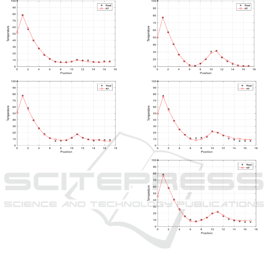
Figure 2: Detection of one heat disturbance using KF. The
heat disturbance is given on the 11
th
grid at 30
0
(top) and
at 56
0
(bottom). The greater heat disturbance given, the
disturbance will be easier to detect since the temperature
in this area is higher than the others.
The heat disturbances on the edges of metal chip
will be easier to detect if the disturbances are on
higher temperature than the boundaries conditions
(figure 4 above), but it’s rather difficult to detect if
one or two of them are in lower temperature (figure
4 bottom). It can be seen that figure 4 (bottom) is
almost same as figure 1. So it’s rather difficult to
detect disturbances in this condition.
The conditions described for Figure 2-4 also
apply to the other number of disturbances i.e. 3, 4,
and 5. Figure 5 show the detection of three, four and
five disturbances with temperature given are listed
on table 1. The disturbance detection also depends
on the number of grids. The more number of grids,
the more accurate the position of detection but these
results are not shown in this paper.
Figure 3: Detection of two disturbances using KF. The
heat disturbances are given on the 10
th
grid at 60
0
and on
the 11
th
grid at 70
0
(above); on the 10
th
grid at 60
0
and on
the 11
th
grid at 30
0
(middle); and on the 10
th
grid at 30
0
and on the 11
th
grid at 60
0
(bottom).
Besides using KF, we also use EnKF to detect
the heat disturbances on the metal chips. We use
some difference numbers of ensembles (i.e.
50,
75, 100, 150) with initial state are generated from
. The disturbance detection using EnKF
result has same conditions as in KF and the figure is
also almost same as Figure 2 – 4. Table 2 shows that
the more ensemble number, the more accurate the
estimation of correction state to the real state.
ICMIs 2018 - International Conference on Mathematics and Islam
12
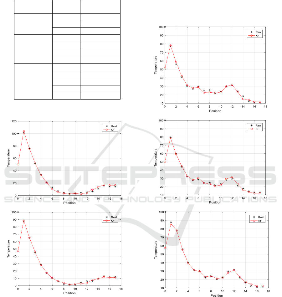
Table 1: Temperatures are given on the disturbances on
figure 5.
Number of
disturbances
Grid
Temperature
Three
6
th
60
0
8
th
50
0
12
th
50
0
Four
6
th
60
0
8
th
50
0
11
th
50
0
12
th
70
0
Five
2
th
90
0
6
th
60
0
8
th
50
0
11
th
50
0
12
th
70
0
Figure 4: Detection of two disturbances on the edges of
the metal chip using KF. The heat disturbances are given
on the 1
st
grid at 170
0
and on the 15
th
grid at 30
0
(above)
and on the 1
st
grid at 70
0
and on the 15
th
grid at 20
0
(bottom).
We will use the average of norm of error
covariance matrix to compare disturbances detection
using EnKF and KF and focus on one and two
disturbances. The comparison result can be seen in
Table 3. It can be seen that the average of norm of
error covariance matrix in EnKF are smaller than the
average of norm of error covariance matrix on KF.
Therefore, for this case the EnKF is more accurate in
the disturbance detection than KF.
Figure 5: Detection of three disturbances (above), four
disturbances (middle) and five disturbances (bottom) using
KF.
Detection of Heat Conduction Disturbance in Cylindrical-Shaped Metal Chip using Kalman Filter and Ensemble Kalman Filter
13
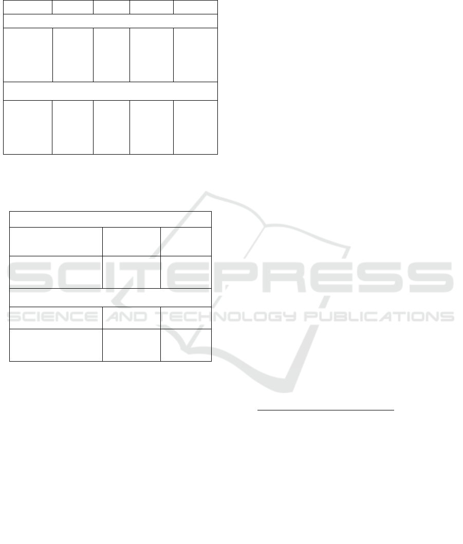
Table 2: The average of norm of error covariance matrices
for different numbers of ensembles in the disturbance
detection using EnKF.
Detection one disturbance
Average of
Norm of
Error
Covariance
matrices
0.00635
0.006
0.00582
0.00574
Detection two disturbances
Average of
Norm of
Error
Covariance
matrices
0.00637
0.006
0.00584
0.00574
Table 3. Comparison of the average of norm of error
covariance matrices between EnKF (
and KF in
detection of one and two disturbances.
Detection one disturbance
EnKF with
KF
Average of Norm of
Error Covariance
matrices
0.00567
0.00944
Detection two disturbances
EnKF with
KF
Average of Norm of
Error Covariance
matrices
0.00566
0.00944
4 CONCLUSIONS
In this study, the KF and EnKF method succeed to
detect the heat disturbances in cylindrical-shaped
metal chip. Detection of heat disturbances has been
carried out for 1–4 disturbances in different
positions. Based on the average of norm of error
covariance matrices, the EnKF is more accurate
detect the disturbance than KF. The heat
disturbances can be detected more clearly if the
temperature of disturbance is large enough,
especially for detection in the edge of chip (close to
inner radius and outer radius). In addition, the more
number of grids, the more accurate the position of
detection.
REFERENCES
Apriliani, E. and Sofiyanti, W., 2011. The Sensitivity of
Ensemble Kalman Filter to Detect the Disturbance of
One Dimensional Heat Transfer, Jurnal Matematika &
Sains, Desember 2011, Vol. 16 (3), pp. 133–139.
Butala, M. D., Yun, J., Chen, Y., Frazin, R. A. and
Kamalabadi, F., 2008. Asymptotic Convergence of
The Ensemble Kalman Filter, 15th IEEE International
Conference on Image Processing.
Carslaws, H. dan Jeager, J., 1959. Conduction of Heat In
Solids, second Edition, London: The Clerendon Press.
Emara-Shabaik, H. E., Khulief, Y. A. and Hussaini, I.,
2002. A non-linear multiple-model state estimation
scheme for pipeline leak detection and isolation.
Proceedings of the Institution of Mechanical
Engineers, Part I: Journal of Systems and Control
Engineering, 216:497.
Evensen, G., 2003. The Ensemble Kalman Filter:
Theoretical formulation and practical implementation.
Ocean Dynamic, 53, 343–367.
Gland, F. L., Monbet, V. and Tran, V. D., 2009. Large
Sample Asymptotics for Ensemble Kalman Filter,
Institut National De Recherche En Informatique En
Automatique.
Hamilton, J. D., 1994. Time Series Analysis, Princeton
University Press, Princeton New Jersey.
Kalman, R. E., 1960. A New Approach to Linear Filtering
and Predictions Problems, Journal of Basic
Engineering 82, 34–45.
Lienhard, J. H., 1930. A heat Transfer Textbook 3
rd
ed./
John H. Lienhard IV and John H. Lienhard V,
Cambridge, MA: J.H. Lienhard V, c2000.
Liu, M., Zang, S. and Zhou, D., 2005. Fast leak detection
and location of gas pipelines based on an adaptive
particle filter. International Journal of Applied
Mathematics and Computer Science, 15(4), pp. 541-
550.
Mandel, J., Cobb, L. and Beezley, J. D., 2009. On the
Convergence of the Ensemble Kalman filter,
University of Colorado Denver CCM Report 278
http://www.arXiv.org/abs/0901.2951.
Tan, M., 2011, Mathematical Properties of Ensemble
Kalman Filter, Dissertation of Faculty of the USC
Graduate School University of California, California.
ICMIs 2018 - International Conference on Mathematics and Islam
14
