
Comparative Study of Spectral Fatigue Life Prediction of LCT
Bottom and Deck Bracket
M. Nurul Misbah
1
, Septia Hardy Sujiatanti
1
, and Raja Andhika Rizki Ramadhani
1
1
Department of Naval Architecture, Faculty of Marine Technology, Institut Teknologi Sepuluh Nopember, Surabaya,
Indonesia
Keywords: Spectral Fatigue, LCT Bottom, Deck Bracket
Abstract: Many LCT ships are converted into passenger ship. The ship is operated and encountered cyclic loading. The
cyclic loading is a vertical bending moment and the horizontal bending moment that randomly applied through
the wave. These bending moments will affect a structural detail to have fatigue. Since these cyclic loadings
are continuously applied and endangered the safety of the ship, then the calculations of fatigue are needed.
Analysis of fatigue capacity using spectral fatigue is taking the variation of headings, load cases and wave
spectrum for each sea state. Headings are started from head sea to the following sea with 45° increment which
are represented headings while the ship is undergoing. The load cases are divided into the full load and full
ballast condition. Wave spectrum is varied and started form 1 m significant wave height to 2,5 m significant
wave height with 0,5 m increment and 5 s to 7 s with increment 1 s for zero-up crossing period. The analysis
result is showing that maximum stress of the ship occurred at heading 135° or quartering sea. Based on the
analysis result, the fatigue life of the ship will be 28 years and 22 years.
1 INTRODUCTION
The ship which located in waters will run into motion
dynamics caused by height and period of the wave.
This motion dynamic resulted in cyclic loads. Cyclic
loads will result in fatigue in a ship structure. An
analysis of fatigue is needed to guarantee the safety
of the ship. One of many methods to predict fatigue
of a ship structure is spectral fatigue with finite
element analysis. This fatigue capacity analysis will
be developed to the fatigue life of a ship structure as
a safety parameter for operation.
This research is carried out to perform technical
calculations of fatigue analysis. These technical
calculations are wave spectrum, structure responses
due to wave, stress at a remote area and fatigue life
analysis. This research used spectral fatigue method.
Spectral fatigue method is a method by using a
statistical approach.
2 LITERATURE REVIEWS
Each sea has its characteristics depend on nature
condition. Sea wave affected by its depth. Therefore,
wave’s form and characteristic are very complex to
explain. Wave basically are differentiated into two
types, sinusoidal and trochoidal. These type of waves
have its complexity so the calculation to determine
actual condition need an approach to visualize
character of waves (Bhattacharyya, 1987). These
statements are formulated in equation (1).
2
0
2
m
m
T
z
(1)
Where,
Tz = period zero up crossing (s)
m0 = spectral moment 0th order
m2 = spectral moment 2nd order.
Wave scatter diagram is a table which has a
correlation between significant wave height (Hs) and
zero-up crossing period (Tz) and notated with a
number of wave incidents. Each table can be
translated by one short-term wave analysis (ABS,
2016).
Misbah, M., Sujiatanti, S. and Ramadhani, R.
Comparative Study of Spectral Fatigue Life Prediction of LCT Bottom and Deck Bracket.
DOI: 10.5220/0008375200910096
In Proceedings of the 6th International Seminar on Ocean and Coastal Engineering, Environmental and Natural Disaster Management (ISOCEEN 2018), pages 91-96
ISBN: 978-989-758-455-8
Copyright
c
2020 by SCITEPRESS – Science and Technology Publications, Lda. All rights reserved
91

2.1 Wave Spectrum
Measured wave data is represented in form of wave
spectrum for further analysis. These spectrums are
represented to each sea-state. The wave spectrums
which are used for analysis have two parameters that
are significant wave height (Hs) and zero-up crossing
period (Tz). These spectrums can be presented in the
Pierson-Moskowitz spectrum (ABS, 2016). These
spectrums are formulated in equation (2).
]
44
)
2
(
1
exp[
5
)
2
(
4
)(
z
T
z
T
Hs
PM
S
(2)
Where,
S(PM) = Pierson-Moskowitz wave spectrum,
Hs = significant wave height (m),
Tz = zero up crossing period (s),
ω = wave frequency (rad/s).
Hasselmann et al found an additional factor for
developed Pierson-Moskowitz wave spectrum. So,
JONSWAP’s spectrum is Pierson-Moskowitz wave
spectrum with peak enhancement factor (Santosa and
Setyawan, 2013). The spectrum in eq. (2) can be
transformed into equation (3).
r
PMJWP
SS
)()(
(3)
Where,
S(JWP) = JONSWAP wave spectrum,
γ = peak enhancement which is 2.5,
r = peak enhancement factor.
2.2 Stress
Stresses occur in a ship are generated from many
sources. Stress which is caused by wave load can be
calculated from bending moments that are caused by
wave horizontally and vertically (Misbah, et.al,
2018). Formulation of stress caused by bending
moments can be explained by equation (4) to equation
(6).
y
I
M
CL
z
H
(4)
z
I
M
NA
y
V
(5)
22
VHT
(6)
Where,
σ = stress (N/m2),
M = bending moment (Nm),
I = inertia moment of section (m3),
z, y = distance of remote area from the neutral axis
or centerline point (m).
Stress analysis was plenteous performed by many
naval architects. One of them is strength analysis.
Strength analysis is divided into two groups, global
and local. For global analysis, Misbah et al, 2018, are
performed on longitudinal strength research and
compared by BKI rules. The analysis is varied by four
load cases that are (a) empty cargo in sagging
condition, (b) empty cargo in hogging condition, (c)
full cargo in sagging condition, and (d) full cargo in
hogging condition. The calculation is performed
using finite element analysis. Results showed that
generated stress are below the permissible stress that
are (a) 72.393 MPa, (b) 74.792 MPa, (c) 129.92 MPa
and (d) 132.4 MPa (Ardianus, 2016). While local
analysis is performed by Ardianus et al, 2017. Local
strength analysis is remoted to transverse bulkhead
between the corrugated bulkhead and conventional
bulkhead. Results showed that corrugated bulkhead is
more effective from generated stress and weight
aspects. The results show the lowest stress and
deformation occurred in corrugated bulkhead are 76.6
N/mm2 with the angle from bulkhead plate 45° and
2.48 mm respectively (Chakrabarti, 1987).
2.3 Response Amplitude Operator
(RAO)
Response Amplitude Operator (RAO) is a character
of structure in regular waves. RAO is a function of
the amplitude of structure motion respected to wave
amplitude (Weibull, 1961). RAO formula can be
written in equation (7).
a
M
Z
M
RAO
(7)
Where,
RAOM = bending moment response amplitude
operator (Nm/m),
M = bending moment (Nm),
Za = wave amplitude.
2.4 Response Spectrum
Structure response in the irregular wave can be
obtained by transforming the wave spectrum into
response spectrum. A response spectrum is defined as
a spectrum of energy density in structure generated by
waves. This spectrum can be generated by calculation
of quadratic RAO and encounter wave spectrum
(Bhattacharyya, 1978).
ISOCEEN 2018 - 6th International Seminar on Ocean and Coastal Engineering, Environmental and Natural Disaster Management
92

)(
2
)(
e
SRAOS
R
(8)
Where,
S(R) = response spectrum,
RAO = response amplitude operator,
S(ωe) = wave spectrum in encounter frequency form.
2.5 Spectral Moment
Further analysis can be statistically done by spectral
moment to determine characteristics of structure
motion due to wave motion. The spectral moment is
used in seakeeping of structure (ABS, 2016). Spectral
moment formula can be done by equation (9).
0
)()(
dSm
R
n
en
(9)
Where,
mn = spectral moment nth order,
S(R) = response spectrum,
ωe = encounter frequency (rad/s).
2.6 Fatigue Life
Fatigue analysis with a spectral method modified
Palgrem-Miner rule into a mathematical model. This
mathematical model is applied to each sea-state
(ABS, 2016). Damage formula will be translated into
equation (10).
M
m
i
i
p
i
f
i
m
m
m
A
T
D
1
)(
00
),()1
2
()22(
(10)
Where,
D = damage,
T = design life,
m = inverse slope,
Γ = gamma function,
λ(m,εi) = Monte Carlo correction,
f0i = event frequency for each sea state,
p0i = event probability of sea state,
σi = standard deviation of stress process.
S-N diagram is obtained by test to several
materials which are fluctuated regular sinusoidal load
applied. These process commonly stated by coupon
testing (Septiana, et.al, 2012).
ANS
m
(11)
Where,
S = stress range (MPa),
m = inverse slope,
N = endurance,
A = fatigue strength coefficient.
Fatigue life calculation can be mathematically
approached with design life and damage factor (ABS,
2016). The formula is showed in equation (12).
D
T
FL
(12)
Where,
FL = fatigue life,
T = design life,
D = damage.
Fatigue life calculation with a combination of load
cases can be done by factor αs or service life of ship
in water in the amount of 0.85 (ABS, 2016).
]
1
...
11
[
1
21 n
s
c
LLL
L
(13)
Where,
Lc = combination fatigue life,
Ln = fatigue life per load cases.
3 Methodology
The methodology of this research based on the theory
on ABS rules and guidance of spectral fatigue
analysis. As mentioned before, started by data and
literature review are needed to be done first. From
theories and data collected, hull modeling is
performed to determine bending moment RAO as
mentioned in equation (7) that will be used to
generate transfer function as mentioned in equation
(4) to equation (6). This performance is needed finite
element analysis. Moreover, probability table and
wave spectrum are modeled with a JONSWAP wave
spectrum according to equation (8).
Furthermore, response spectrum is generated for
each sea-state as mentioned in equation (8). These
responses are analyzed statistically with spectral
moment based on equation (9). Damage calculation
performed with a combination of the spectral
moment, correction and S-N diagram started from
equation (9) to equation (12). The final step of this
research is to determine the fatigue life of a
combination of all load cases based on equation (12)
to equation (13).
Comparative Study of Spectral Fatigue Life Prediction of LCT Bottom and Deck Bracket
93
4 Result and discussion
4.1 Section Modulus and Weight
Distribution
Section modulus can be calculated by analyzing part
to the part based on baseline or deck and centerline
vertically and horizontally. Outputs of this calculation
are INA, z1 ICL, and y1. The section modulus
calculation can be seen in Table 1.
Table 1. Section Modulus of Ship
Item
Value
Unit
I
NA
142196979,6
cm
4
I
CL
1460805765
cm
4
z
1
170,5
cm
y
1
0
cm
Weight distribution for full cargo and empty cargo
load cases are obtained from stability document. The
result shows in Table 2.
Table 2: Weight Distribution
Data
Unit
Load Case
Full
Empty (Ballasted)
Weight Distribution
LWT
ton
712,1
712,1
DWT
ton
811
638
Total
ton
1523,1
1350,1
Buoyancy & Mass Center
T
m
2,351
2,118
VCB
m
1,25
1,13
LCB
m
25,71
25,93
VCG
m
4,19
3,15
LCG
m
25,75
25,96
Displ. & Vol. Displ
Δ
ton
1523,1
1350,1
Vol. D
m
3
1485,951
1317,171
4.2 Hull Modelling
S-N Diagram selection is based on the high value of
SCF (Stress Concentration Factor) for safety reason.
The result showed in Table 3. The remote area is
based on midship (Fr. 15) and outer bracket.
Table 3. S-N Diagram Parameter
Parameter
Value
m
3
A
4,31
10
11
In this research, fatigue analysis takes focus on
bracket connection between longitudinal and web
frame. This remote area has highest SCF (1.03 times
of nominal stress). Hull modelling to be carried out
by using finite element software. The result shows
that the bending moment has a constant value in 1,7
m size for elements. The illustration of the finite
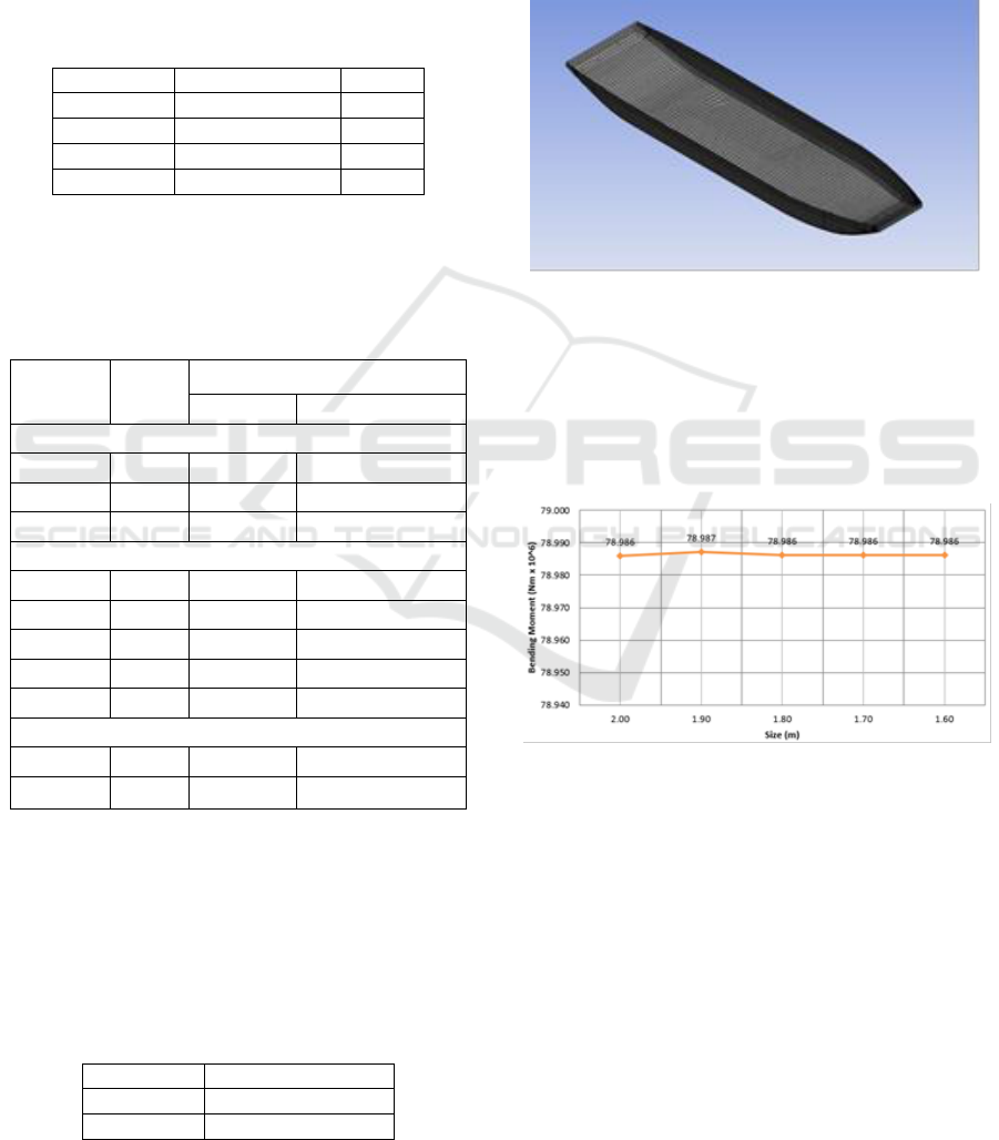
element model shows in Figure 1.
Figure 1: Ship Hull Finite Element Model
Figure 2 shows that the ship’s hull is divided into
panel elements. These panels are used for finite
element analysis. According to Figure 2, bending
moment generated from the model has no significant
difference between 3rd run and 4th run respected to
element size. So, the convergent element is 1,7 m.
Figure 2: Element Convergence
4.3 Wave Data
Wave scatter diagram is composed of significant
wave height (Hs) and zero-up crossing period (Tz).
The processed data presented in Table 4.
ISOCEEN 2018 - 6th International Seminar on Ocean and Coastal Engineering, Environmental and Natural Disaster Management
94
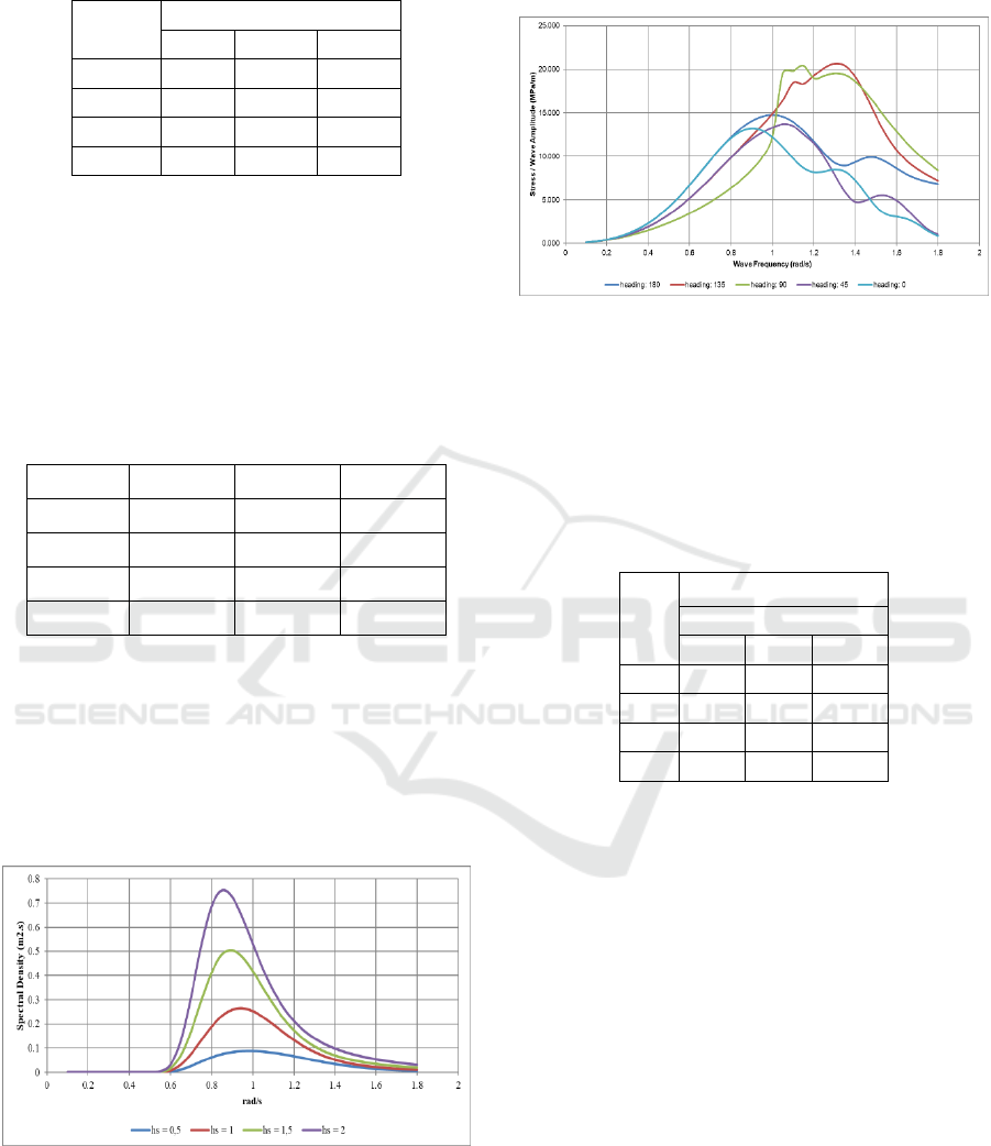
Table 4: Bali Strait Wave Data (Yustiawan and Suastika,
2012)
Hs (m)
Tz (s)
5
6
7
1.0
5887
58061
14947
1.5
0
3856
8493
2.0
0
2
460
2.5
0
1
18
According to Table 4, it can be seen that at Hs = 1
m and Tz = 6 s is a dominant sea-state at Bali Strait.
So, the fatigue analysis will be dominant from this
sea-state.
Table 5 shows that the highest probable heading
of the wave is from a southeast area with 44.244% of
total recorded heading.
Table 5. Bali Strait Wave Heading Data (Yustiawan and
Suastika, 2012)
Heading
P
heading
Heading
P
heading
E
0.003%
W
1.254%
SE
44.244%
NW
0.000%
S
25.672%
N
0.003%
SW
28.820%
NE
0.003%
4.4 Wave Spectrum
Wave spectrum is generated based on equation (3)
and represented with the correlation between spectral
density and wave frequency. Result for one of the
spectrum with maximum spectral density is 0.75 m2s
as shown in Figure 3.
Figure 3: Wave Spectrum at Zero-up Crossing 5
According to equation (4) to equation (7), RAO
stress is dominated by stress from quartering sea
(135°) as shown in Figure 4 presented by red colored.
It caused by a combination between vertical and
horizontal stress, so the resultant of stress will happen
at quartering sea.
Figure 4: RAO Combination of Vertical and
Horizontal Stress at Bottom Full Cargo
A generated spectral moment from structure
response caused by wave shows that maximum value
at Hs = 2.5 m. Table 6 is one of many spectral
moments resulted.
Table 6: Spectral Moment 0th Order of Full Cargo Load
Case at Bottom Bracket
Hs
(m)
Heading 180°
Tz (s)
5
6
7
1
7,1
10,3
12,3
1.5
18,1
27,4
33,4
2
30,9
50,0
63,0
2.5
43,2
74,0
96,6
4.5 Fatigue Life
From generated result before, the damage calculation
can be obtained. Damage capacity is the main factor
in fatigue. Damage distribution can be analyzed by
Table 7. Based on Table 7, bracket at the deck with
full cargo load will have the highest value of damage
so it has the shortest life of fatigue. Furthermore, the
combination of load case can be coupled based on
equation (13). The fatigue life calculation result
shows in Table 8.
Comparative Study of Spectral Fatigue Life Prediction of LCT Bottom and Deck Bracket
95

Table 7. Damage and Fatigue Life
Bracket
Location
Load case
D
actual
Fatigue
life (year)
Bottom
(Rohmadhana
and
Kurniawati,
2016)
Full cargo
0.496
20.13
Empty
cargo
0.319
31.30
Deck
Full cargo
0.624
16.01
Empty
cargo
0.404
24.75
Table 8: Combination Fatigue Life
Bracket
Location
Load
case
D
actual
Combination
fatigue life
(year)
Bottom
(Rohmadhana
and
Kurniawati,
2016)
Full
cargo
0.496
28.83
Empty
cargo
0.319
Deck
Full
cargo
0.624
22.88
Empty
cargo
0.471
Based on Table 8 it can be seen that the shortest
fatigue life of the structure is on the deck with the
fatigue life 22 years while at the bottom is 28 years.
It is caused by the deck is the farthest distance from
the neutral axis of the ship.
5 CONCLUSION
According to the analysis and results, this research
can be concluded into:
1. Fatigue life of each case at the bottom is 20
years and 31 years for full cargo and empty
cargo respectively where each load cases are
acceptable according to ABS (20 years).
2. Fatigue life of deck structure has the shortest life
approximately 16 years and 24 years for full
cargo and empty cargo respectively where full
cargo condition is not acceptable according to
ABS (20 years).
3. Both fatigue life of combinations of load cases
at the bottom and at deck are 28 years and 22
years respectively where it is acceptable
according to ABS (20 years) with factor 0.85
represented as the service life of the ship.
REFERENCES
A. Yustiawan, & K. Suastika, Fatigue Life Prediction
of Keel Buoy Tsunami Structure with Spectral
Fatigue Analysis Method, Jurnal Teknik ITS Vol.
1 No. 1 ISSN:2337-3539, Surabaya: Institut
Teknologi Sepuluh Nopember, (2012).
American Bureau of Shipping (ABS), Spectral-Based
Fatigue Analysis for Vessels, Houston: American
Bureau of Shipping (2016).
Ardianus, S.H. Sujiatanti, & D. Setyawan, Analisa
Kekuatan Konstruksi Sekat Melintang Kapal
Tanker dengan Metode Elemen Hingga. Jurnal
Teknik ITS 6 (2), G183-G188, ISSN: 2337-3539,
Surabaya: Institut Teknologi Sepuluh Nopember.
B. Santosa, & D. Setyawan, Lecture Handout, Ship
Structure and Strength, Surabaya: Institut
Teknologi Sepuluh Nopember (ITS), (2013).
D. Septiana, Soeweify, A Imron, Estimated Fatigue
Life on the Tanker Ship Bracket Based on
Common Structural Rules, Jurnal Teknik ITS
Vol. 1 No. 1 ISSN:2337-3539, Surabaya: Institut
Teknologi Sepuluh Nopember, (2012).
F. Rohmadhana, & H.A. Kurniawati., Technical and
Economic Analysis of Conversion of Landing
Craft Tanks (LCT) to Crossing Motorboats
(KMP) Type Ro-ro for Ketapang Routes
(Banyuwangi Regency) - Gilimanuk (Jembrana
Regency), Jurnal Teknik ITS Vol. 5 No. 2
ISSN:2337-3539, Surabaya: Institut Teknologi
Sepuluh Nopember, (2016).
M. Huda, & B. Santosa, Analysis of Estimated Age
of Structure on the 10 GT Catamaran Fish Ship
Using Finite Element Method, Jurnal Teknik ITS
Vol. 1 No. 1 ISSN:2337-3539, Surabaya: Institut
Teknologi Sepuluh Nopember, (2012).
M. N. Misbah, D. Setyawan, & W. Murti Dananjaya.,
Construction Strength Analysis of Landing Craft
Tank Conversion To Passenger Ship Using Finite
Element Method, Journal of Physics: Conference
Series. 974. 012054. 10.1088/1742-
6596/974/1/012054, (2018).
M. Rusdi., M. N. Misbah., T. Yulianto., Analysis of
Fatigue Life on Oil Tanker Bracket with Sloshing
Load, Jurnal Teknik ITS Vol. 7 No. 1 ISSN:2337-
3539, Surabaya: Institut Teknologi Sepuluh
Nopember, (2018).
R. Bhattacharyya, Dynamic of Marine Vehicle, U.S.
Naval Academy, Annapolis: Marryland. (1978).
S. Chakrabarti, Hydrodynamic of Offshore
Structures, Boston, USA: Computational
Mechanics Publications Southampton (1987).
W. Weibull, Fatigue Testing and Analysis of Results,
Oxford: Pergamon Press, (1961).
ISOCEEN 2018 - 6th International Seminar on Ocean and Coastal Engineering, Environmental and Natural Disaster Management
96
