
Develop Inverse Models to Track Environmental Pollutants
Using Mass Conservation Law for both Normal and
Anomalous Transport
S Dawley
1
, Y Zhang
1,*
, H G Sun
2
and C M Zheng
3
1
Department of Geological Sciences, University of Alabama, Tuscaloosa, AL 35487,
USA
2
State Key Laboratory of Hydrology-Water Resources and Hydraulic Engineering,
College of Mechanics and Materials, Hohai University, Nanjing 210098, China
3
School of Environmental Science & Engineering, Southern University of Sciences
and Technology, Shenzhen 518055, China
Corresponding author and e-mail: Y Zhang, yzhang264@ua.edu
Abstract. When pollutants are found in the environment (such as indoor air, land surface,
rivers, and aquifers), one of the major challenges is to identify the source position(s) or the
release history of the pollutants. This issue can be most efficiently addressed by the inverse
modelling approach, which can directly back track the pollutant’s previous location(s) given
the current location and travel time, o r calculate the pollutant’s release history given the
current and initial positions. It is, however, not trivial to develop the inverse model. Most
importantly, both normal and anomalous transport can occur for pollutants in different
systems, and how to build inverse models to efficiently back track these quite different
transport dynamics using a unified, physically reasonable approach remains a historical
challenge. This study develops inverse models for pollutants undergoing either normal
transport or super-diffusive, anomalous transport using the well-known and universal mass
conservation law. Results show that the combination of the mass balance law with reversing
time and the standard Tayler series expansion leads to the inverse model for normal transport,
while the mass balance law combined with the Grünwald approximation of fractional
derivative builds the inverse model for anomalous transport. Numerical solvers are also
developed to approximate the forward and inverse models, so that this study provides
convenient tools to identify environmental pollutants with a wide range of intrinsic
heterogeneity.
1. Introduction
World-wide contamination such as the global and continuous deterioration of fresh water resources is
jeopardizing our environment, economy, and society. When pollutants are found in the environment,
one of the major concerns is its original source location if the travel time or age of the pollutants is
known, or the release history of the pollutants if the source is known [1]. Environmental management
and contaminant remediation require previous properties of the pollutant, which can be most
efficiently obtained using the inverse modeling approach [2]. The inverse models can directly back
Dawley, S., Zhang, Y., Sun, H. and Zheng, C.
Develop Inverse Models to Track Environmental Pollutants Using Mass Conservation Law for Both Normal and Anomalous Transport.
In Proceedings of the International Workshop on Environmental Management, Science and Engineering (IWEMSE 2018), pages 323-330
ISBN: 978-989-758-344-5
Copyright © 2018 by SCITEPRESS – Science and Technology Publications, Lda. All rights reserved
323

track the position where the pollutants originated, or the backward time when the pollutants first
entered the system. Although the inverse models can be extremely helpful, it is not trivial to develop
reliable inverse models. The sensitivity analysis approach proposed by Neupauer and Wilson [2] has
been regarded as the most reliable method to build the inverse models for Fickian-diffusive pollutants;
see the review by Liu and Zhai [3] and Cheng and Jia [4].
There are however two historical challenges in the sensitivity analysis approach. Firstly, it is a
complex statistical approach, where the multi-step statistical analysis (i.e., the adjoint probability and
marginal performance) is difficult to be interpreted physically by most users. Second, it was applied
mainly for pollutants undergoing normal transport due to Fickian diffusion (where the variance of
pollutant displacement increases linearly in time) in relatively homogeneous media. Anomalous
transport with a nonlinear evolution of the variance of pollutant displacement, however, has been
increasingly documented in real-world systems which can be heterogeneous with multi-scale intrinsic
heterogeneity, such as rivers, soil, and aquifers; see for example, Ref. [5~7], among many others.
This study aims at developing a physically sound approach based on the mass conservation
(which should be valid for both the forward-in-time and backward-in-time processes) to derive
inverse models for pollutants in both relatively homogeneous and strongly heterogeneous media.
Particularly, we consider super-diffusive, anomalous transport of pollutants along preferential flow
paths, such as fractures or interconnected ancient channels in subsurface that can substantially
enhance the motion of pollutants and therefore pose a high risk to the ecosystem.
The rest of this work is organized as follows. In Section 2, we apply the mass conservation law
combined with the standard Taylor series approximation to derive the inverse model for pollutants
undergoing normal transport. This methodology is then extended for anomalous transport in Section
3. Section 4 shows the numerical solver for the forward and inverse models with numerical examples
and validations, and the relationship between the models is then discussed in Section 5. Conclusions
are finally drawn in Section 6.
2. Development of inverse model for normal transport
For simplicity, here we consider the pollutant particle (in forward-in-time) moves or backward
probability expands in one direction (x). Note that the following methodology can be conveniently
extended to multiple dimensions, since it is not dimension limited.
Let M
i
be the number of particles (which can carry backward probabilities in the inverse model) in
cell i, the particle density in this cell is then given by:
, (1)
where
[L
3
] is the volume of cell i. If the particle generally moves from cell i to cell i+1 under
ambient conditions, then the particle number flux from cell i+1 to cell i per unit area and per unit
time in the backward-in-time process is [8]:
, (2)
where the parameter
[dimensionless] represents the difference in probabilities when particles jump
forward and backward along the x-axis (
); [L
2
] is the area of the cell normal to the x-axis; R
[T
-1
] is the number of jumps per unit time for each particle; and [L] is the cell length. Using the
following Taylor series approximation
, (3)
where denotes the truncation error, and s denotes the backward time. Equation (2) can then be
written as:
IWEMSE 2018 - International Workshop on Environmental Management, Science and Engineering
324

. (4)
When , it is obviously that
(where represents the mean drift). Also,
according to Fick’s law [8], one has
(where D denotes the dispersion
coefficient). The above equation becomes:
. (5)
We assume that the total number of particles remains stable during jumps; or in other words, we
only consider the transport of conservative pollutants. The conservation of particle mass also means
the conservation of the number of particles. Substituting equation (5) into the mass conservation
equation (for backward-in-time processes)
, (6)
we obtain the inverse model for normal transport in relatively homogeneous systems:
. (7)
The above formula is the well-known Kolmogorov backward equation, which is also the inverse
model of the 2
nd
-order advection-dispersion equation (ADE) derived by Neupauer and Wilson [2]
using the sensitivity analysis based, complex statistical approach mentioned above. The forward-in-
time ADE model takes the form:
. (8)
Compared to the forward-in-time ADE model (8), the inverse model (7) reverses the flow field
while keeping the dispersive (backward probability) flux term unchanged (which is called “self-
adjoint” by Neupauer and Wilson [2]) to back track pollutant source or age. The “self-adjoint”
dispersion in the inverse model (7) is due to the physical interpretation of backward tracking, because
the backward location (or travel time) probability distribution function (PDF) expands when moving
backward further, representing the increasing uncertainty for the identification of the pollutant’s
source position (or age) with an increase backward time s (or the backward travel distance). Here the
backward location PDF provides the probability for all upstream locations being the source position
for a given detection of pollutants with a known age. The backward travel time PDF describes the
probability of a certain time required for the pollutant particle to travel between the detection well
and its known source location. Both above PDFs can be calculated from the inverse model (7), using
the particle tracking approach discussed in Section 4.
3. Development of inverse model for anomalous transport
The forward-in-time, spatial fractional advection-dispersion equation (fADE) was derived by
Schumer et al. [8] using the mass conservation approach similar to the one used above, except for the
standard Taylor series expansion (3) (which is no longer valid for anomalous jumps). The
generalized Taylor series proposed by Osler [9] was applied by Schumer et al. [8] to replace formula
(3) and then derive the fADE model (see for example, equation (10) in Schumer et al. [8]):
, (9)
where the operator
denotes the Reimann-Liouville fractional derivative with order (j is
an integer number) and skewness [dimensionless] ( ), and [dimensionless] is the
Gamma function. The second equality in (9) can be used to replace the standard Taylor series
Develop Inverse Models to Track Environmental Pollutants Using Mass Conservation Law for Both Normal and Anomalous Transport
325
expansion (3) and derive the inverse fADE model. However, the above formula (9) is questionable in
definition [10]. In addition, it cannot be used to capture the important drift displacement of pollutant
particles (since the second equality in (9) does not contain the first-order term of
), requiring
the additional and debatable assumption of Galilei variant [11,8].
Here we fix the above issue by adopting the zero-shifted Grünwald approximation proposed by
Meerschaert and Tadjeran [12]:
, (10)
where q [dimensionless] ( ) is the scale index indicating the order of fractional
differentiation; the symbol
denotes the (negative) Riemann-Liouville fractional
derivative (note that the negative fractional derivative is selected here since the inverse process
exhibits an opposite skewness for the preferential displacement compared to its forward-in-time
counterpart; see our recent work in [13]); N [dimensionless] is a sufficiently large number of grid
points in the downstream direction; and
[dimensionless] is the Grünwald weight defined by:
. (11)
Inserting (11) into (10), and then approximating the negative fractional derivative using the first
two major terms (note that the contribution from the remaining terms in (10) is negligible due to their
small weights [14]), we have
, (12)
which can be re-arranged as:
. (13)
The approximation (13) reduces to equation (3) when , implying that the Grünwald
approximation (10) can be used to obtain the generalized Taylor series expansion.
Combining equations (13) and (2), and then using the mass conservation law (6), we obtain the
inverse model for pollutants undergoing super-diffusive anomalous transport:
, (14)
which leads to the following inverse model if all parameters are constant:
, (15)
where the index [dimensionless].
The forward-in-time counterpart of (15) is the following fADE model [13]:
, (16)
which has been widely used to quantify pollutant/material transport in heterogeneous systems
[15~18].
4. Numerical solutions and validations
The above forward and inverse models can be approximated by a particle-tracking based, fully
Lagrangian solver. First, for the forward-in-time ADE model (8), we build the following Langevin
equation, which describes a Markov process for particle tracking:
IWEMSE 2018 - International Workshop on Environmental Management, Science and Engineering
326

, (17)
where
[L] is a differential distance of travel,
is the current particle location, [T] is
a differential unit of time, and denotes independent normally distributed random variables with
zero mean and unit variance. Here we assume D is constant; otherwise an additional drift,
,
should be added in (17) to account for the impact of the spatial variation of D on particle dynamics. It
is also noteworthy that here the velocity can vary in space, although this variation is not needed for
a one-dimensional model. The following Langevin equation corresponds to the inverse ADE model
(7):
, (18)
where [T] is the differential unit of time for backward tracking.
Second, for the forward fADE model (16), the corresponding Langevin equation is:
, (19)
where
denotes a Lévy α-stable random noise with maximally positive skewness, one scale,
and zero shift [19]. The Langevin equation for the inverse fADE model (15) takes the form:
, (20)
where
denotes a Lévy α-stable random noise with maximally negative skewness, one scale,
and zero shift [19]. After obtaining the trajectory of each random walker, the particle number density
provides the solution of each transport model, which can be converted to the backward location and
travel time PDFs. This is because the spatial distribution (i.e., the resident number density) of
particles at a given time is related to the backward location PDF, while the flux number density of
particles at a given control plane is related to the backward travel time PDF [2,13].
Eularian solvers can also be developed to approximate the above forward and backward models,
by extending for example the implicit Eularian finite difference scheme developed by Meerschaert
and Tadjeran [12].
The above numerical solvers were tested extensively. A few examples are shown in Figure 1,
where the model parameters are as follows: , v*=1, and D*=5. In Figure 1b, the inverse 2nd-
order ADE (7) is also shown for comparison (whose solution is multiplied by a factor 0.5 for a better
visual). The four crosses in Figure 1b, which describe four possible (backward) point source
positions with different probabilities and can be linked with the forward resident concentration
showing in Figure 1a, illustrate the equivalence between the forward and the backward location PDFs
for the fADEs. This equivalence confirms for the first time the result in Zhang et al. [20], who found
that the backward location PDF should be an image of (and therefore should equal) the forward
location PDF for super-diffusive pollutants when the backward time s and the forward time t have the
same magnitude.
Develop Inverse Models to Track Environmental Pollutants Using Mass Conservation Law for Both Normal and Anomalous Transport
327
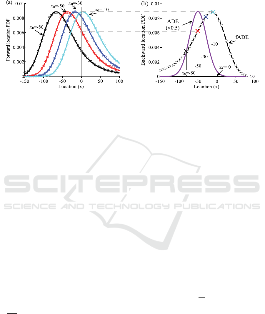
Figure 1. Numerical experiments. (a) Forward location PDF for model (16) at a forward time
t = 50 for four possible source locations (x
0
). (b) The corresponding backward location PDF
for model (15) at time s = 50, from the detection well located as x
d
= 0. Circles denote the
Lagrangian solutions (with 10
6
particles and 10
2
time steps), and lines denote the Eulerian
solutions. See the main text for other model parameters.
In addition, the backward location PDF for normal diffusion distributes symmetrically in space
(around the most likely source position at ) (Figure 1b), implying the equal
probability for pollutant particles to jump downstream and upstream due to Fickian diffusion during
each motion. The backward location PDF for anomalous diffusion, however, is highly skewed with a
prolonged tail toward the upstream zones (Figure 1b), revealing the contribution of potential
preferential flow paths on pollutants that can convey pollutant particles from a long distance
upstream in a short time.
5. Discussion
The forward/backward models for anomalous transport can be reduced to the models for normal
transport. For example, when (representing the end member of the media, which is the
homogeneous medium), the inverse model (14) for heterogeneous media reduces to model (7) for the
relatively homogeneous media. In addition, when , the forward model (16) reduces to the
classical ADE model (8) with constant parameters. Hence, the forward/backward models for
anomalous transport contain the forward/backward ADE models as special cases. “Normal” transport,
therefore, might be regarded as an end member of anomalous transport. Or in other words, all real-
world systems are heterogeneous (note that strictly speaking, there is no absolutely homogeneous
system in nature), and the “homogeneous” system might just be an ideal case with a negligible
degree of heterogeneity [21].
It is also noteworthy that the Langevin equation for the forward/backward anomalous transport
cannot be directly linked to those for normal transport. For example, in equation (19), although the -
stable random variable
(which is on the same order as
in equation (17) when
), the -stable Lévy motion described by (19) has a different scaling factor (
) than that
(
) in the Brownian motion in (17). This discrepancy is simply due to the fact that a standard
stable with is not standard normal [22]. Numerical experiments (not shown here) do confirm
that the solution of (19) (or (20)) with is similar to (17) (or (18)), as expected.
6. Conclusions
Long-term environmental management, protection, and remediation require the previous properties
of pollutants detected in the natural media (such as air, rivers, ocean, land slope, soil, and aquifers),
IWEMSE 2018 - International Workshop on Environmental Management, Science and Engineering
328

including for example the pollutant source locations and the release time, which can be quantified
mathematically by the backward location probability density function and the backward travel time
probability density function, respectively. Both PDFs can be obtained conveniently and reliably by
solving the appropriate inverse model, whose derivation however remains a challenge. Transport
process for pollutants can also exhibit either normal behaviour (in ideal, homogeneous media) or
anomalous behaviour (in heterogeneous media). There is lack of a physically clear method that can
build inverse models for a wide range of transport behaviours , which motivated this study. Three
major conclusions are drawn from this work.
First, the universal mass conversation law, when combined with the appropriate Taylor series
expansion, can build the inverse models for both normal and anomalous transport. The standard
Taylor series expansion leads to the inverse model for normal transport following the classical 2
nd
-
order advection-dispersion equation, while a corrected, generalized Taylor series expansion (owning
to the Grünwald approximation) is needed to derive the inverse counterpart for the fractional
advection-dispersion equation model that has been widely used by hydrologists to quantify super-
diffusive anomalous transport in natural geological deposits.
Second, cautions are needed when deriving the inverse models using the mass conversation law.
The time needs to be reversed, and the dispersive jumps of particles also need to be skewed to the
opposite direction if the jumping probability along the downstream and upstream directions is no
longer symmetric. The spatial direction, however, remains unchanged, since the drift is now reversed.
Third, a particle-tracking based Lagrangian solver is developed and validated to approximate all
the forward and inverse models. Hence, this study may provide convenient tools to identify
environmental pollutants. Real-world applications will be conducted to check the feasibility of the
proposed technique in a future study.
Acknowledgement
This work was partially supported by the National Natural Science Foundation of China under grants
41628202, 41330632, and 11572112. This paper does not necessarily reflect the views of the funding
agency.
References
[1] Atmadja J and Bagtzoglou A C 2001 Environ. Forensics 2 205
[2] Neupauer R M and Wilson J L 2001 Water Resour. Res. 37 1657
[3] Liu X and Zhai Z 2007 Indoor Air 17 419
[4] Cheng W P and Jia Y F 2010 Adv. Water Resour. 33 397
[5] Meerschaert M M, Zhang Y and Baeumer B 2008 Geophy. Res. Lett. 35 L17403
[6] Neuman S P and Tartakovsky 2009 Adv. Water Resour. 32 670
[7] Le Borgne T, Dentz T, Davy P, Bolster D, Carrera J, de Dreuzy J R and Bour O 2011 Phys.
Rev. E 84 015301(R)
[8] Schumer R, Benson D A, Meerschaert M M and Wheatcraft S W 2001 J. Contam. Hydrol. 48
69
[9] Osler T J 1971 SIAM J. Math. Anal. 2 37
[10] Jumarie G 2006 Comput. Math. Appl. 51 1367
[11] Metzler R and Klafter J 2000 Phys. Rep. 339 1
[12] Meerschaert M and Tadjeran C 2004 J. Comput. Appl. Math. 172 65
[13] Zhang Y, Meerschaert M M and Neupauer R M 2016 Water Resour. Res. 52 2462
[14] Zhang Y, Benson D A, Meerschaert M M and LaBolle E M 2007 Water Resour. Res. 43,
W05439
[15] Zhou L and Selim H M 2003 Soil Sc. Soc. Am. J. 67 1079
[16] Huang Q, Huang G and H Zhan 2008 Adv. Water Resour. 31 1578
Develop Inverse Models to Track Environmental Pollutants Using Mass Conservation Law for Both Normal and Anomalous Transport
329

[17] Bradley D N, Tucker G E and Benson D A 2010 J. Geophy. Res. 115 F00A09
[18] Chao K Y, Muniandy S V, Woon K L, Gan M T and Ong D S 2017 Org. Electron. 41 157
[19] Samorodnitsky G and Taqqu M 1994 Stable Non-Gaussian Random Processes (New York:
Chapman & Hall)
[20] Zhang Y, Sun H G, Lu B Q, Garrard R and Neupauer R M 2017 Adv. Water Resour. 107 517
[21] Fogg G E and Zhang Y 2016 Water Resour. Res. 52 9235
[22] Zhang Y, Benson D A, Meerschaert M M and Scheffler H P 2006 J. Statis. Phys. 123 89
IWEMSE 2018 - International Workshop on Environmental Management, Science and Engineering
330
