Forecasting Electricity Consumption of Appliances based on

the Additive Factor Hidden Markov Model

Q Gao

, Y Su

, L B Wu

1, 2, *

and Y Zhou

1,2

Fudan University, School of Computer Science, Yangpu District, Shanghai

200433, China;

Fudan University, School of Economics, Yangpu District, Shanghai 200433,

China;

State Grid Shanghai Municipal Electric Power Company, Pudong New District,

Shanghai, China

Q Gao and Y Su are the first authors.

Corresponding author and e-mail: L B Wu, wulibo@fudan.edu.cn

Abstract. Accurately forecasting the electricity demand and feedback on separate

appliances can lead to natural energy-saving behaviors and higher energy efficiency. In

this paper, a supervised additive factor hidden Markov model including the exogenous

influencing factors is developed to forecast the electricity usage of appliance in building

based on the hourly data, where the model is trained with the first part of appliances data

to get optimized parameters and tuned with aggregate electricity data in forecasting. The

model successfully forecast the usage of all appliances for a mall building and the

accuracies for appliances are all larger than 60%, which is higher than most similar

analyses, especially same frequency data analysis. By adding the influence factors, the

AFHMM model gives a more accurate result in lower frequency data, which can be

widely used in energy monitoring of buildings.

1. Introduction

Environmental pollution and shortages of resources are two continuously concerning but unresolved

problems of the past decades, which are related to the sustainable development of the world.

Developing energy-saving technologies to improve the efficiency of energy utilization is an

important and effective strategy to reduce wastes of resources and emissions of pollutants. Among

the numerous energy-saving strategies, accurately forecasting the electricity demand of each

appliance and feedback to users let the users know their detailed electricity behaviors and lead to

natural energy-saving behavior and higher energy efficiency without affecting normal life, especially

for commercial buildings [1,2]. Ref. [3] finds that the energy-saving ratio grows fast with more

feedback information [4-6], where real-time information about appliances can even approach 50%

[6] energy-saving.

There are two problems for the forecasting of the usage of appliances, data frequency and models.

First, the traditional forecasting analyses [7-10] always use electricity data monthly or yearly in

China, which cannot satisfy the demand to separate the behaviors of appliances. Second, the models

Gao, Q., Su, Y., Wu, L. and Zhou, Y.

Forecasting Electricity Consumption of Appliances based on the Additive Factor Hidden Markov Model.

In Proceedings of the International Workshop on Environmental Management, Science and Engineering (IWEMSE 2018), pages 193-200

ISBN: 978-989-758-344-5

193

of other analyses [3] in forecasting the usage of appliances can only apply to data with frequency in

kHz level or get a result with accuracy lower than 55% for hourly data [11]. In this paper, we develop

a new model by considering the influences for the additive factor hidden Markov model (AFHMM)

[12], which can forecast the electricity consumption of appliances with aggregate electricity data in

long-term and get a high accurate result for hourly data [13] collected by smart meters in Shanghai.

The method is possible to be shared to buildings without collectors of appliances and used in energy

monitoring.

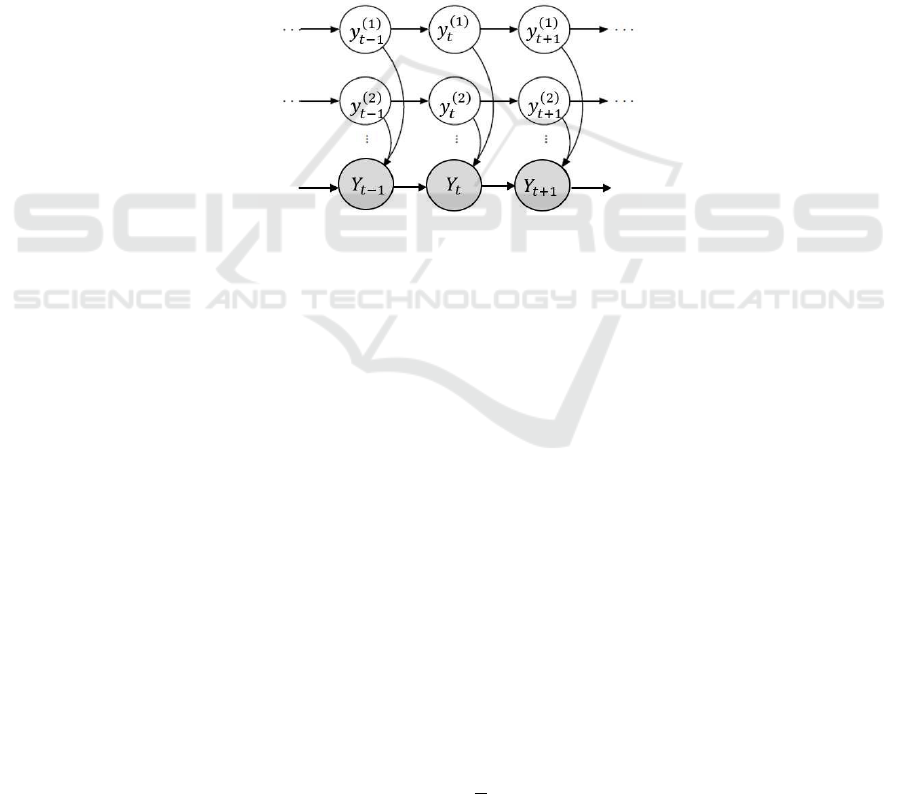
2. Model

The AFHMM is shown in Figure 1 [12]. Suppose that every appliance is a hidden Markov process

with multiple different states and is represented by a submodel, where the electricity consumption for

each state is influenced by many exogenous factors such as weather, outdoor temperature, holiday,

night and others. While the aggregate electricity consumption, i.e., the summarization of the usage of

all appliances, is also a hidden Markov process. The states of the additive model are the combination

of the states of submodels and the number of states are the product of all the numbers of submodels.

Figure 1. Additive factor hidden Markov model.

The analysis process is split into the following several steps:

1 Separate the electricity data of the appliances into two continuous parts: the training set and the

testing set. The training set is used for optimizing the model with data of aggregate and separate

electricity consumption and all influencing factors, while the testing set is used for testing the effect

and accuracy of the model only with data of aggregate electricity consumption and influencing

factors.

2 Get the parameters of each submodel to construct the AFHMM model with all aggregate data.

Get the state of aggregate data in a test set by observations, and decode it to every appliance.

3 Predict the expected value of each appliance in a test period by training the model without

observations. Repair the expected value of each appliance by aggregate observations and states from

the additive HMM model.

4 Compare the measured and forecasting data by calculating the accuracy of model training and

testing.

2.1. AFHMM model and HMM model

Suppose that the probability of total usage at one state satisfies a normal distribution and that the

expected value is the summarization of corresponding states of submodels , while the expected values

of submodels are linear functions of influencing factors and the probabilities also satisfy normal

distributions:

     

1: 1:

()

( ( )) ~ ( ( ), ( ))

N i N

p Y S N y S S







(1)

IWEMSE 2018 - International Workshop on Environmental Management, Science and Engineering

194

       

     

( ) ( )

( ) ( ) 2

( ) ( ) ( ) ( | )

( ( )) ~ ( ( ), ( ))

i i i i

t i i t t

i i i

y S c S S O f O S

p y S N y S S





   

(2)

where

is the aggregate value,

is the number of appliances,

 

is the state of

-th appliance

at time

 

()

is the expected value of

-th appliance under state

 

at time

and

the outer influencing factors. The expected value of each appliance is related with many other

variables and they are measured independently with electricity. The number of states for the

-thi

appliance

()i

is obtained by Bayesian information criterion (BIC) [14] and the EM method. Each

appliance includes initial state probability, transition matrix, outer effects, and normal distribution

sigma.

2.2. Determine the AFHMM model

The parameters of additive FHMM model is obtained by combining the parameters of each appliance.

The total number of states is the product of that of all appliances. And the state probability, transition

matrix and state distribution parameters are Kronecker products [15] of separate appliances.

   

 

   

1: 1:

( ) ( ) ( )

( | ) | ,

N i N i

i i k

p S Y p S y S S m





  





(3)

where

 

( | )

p S Y

is the posterior probability of state

 

1: N

under the condition of aggregate

usage

at time

for the system, and

 

( ) ( )

p S y

is the similar probability for

-th

appliance, where the state of system is a Kronecker combination of all appliances. By fixing the

parameters, the conditional state distribution of the AFHMM model of the test period can be obtained

by repeating the following processes:

     

 

   

 

1: 1: 1:

1: 1:

( | 1) ( | )

( | 1) ( ( ))

( | )

( ( ))

N N N

p S t p S Y

p S t p Y S

p S Y

p Y S



  







(4)

where

 

1: N



is the transition matrix for the entire model. By decoding the aggregate state

distribution with the method of inverse equation (5), the state of each appliance

 

p S Y



each time in future is obtained.

2.3. Predict and adjust for separate appliances

For every appliance, there is no electricity data in the testing set. The expected values can be

obtained only by the training model:

 

     

 

( ) ( ) ( ) ( ) ( )

| | |

( ) ( | ) | ( )

i i i i

i i i h i i h

i i i i

i i i i i

t h t h t h t h

p S t h p S y p S y

y S f O S y p S t h y S

   

   

  



，

(5)

where

is the length of training set,

 

()

( | )

f O S



is the linear function of influencing

factors



from equation (2). To predict

stage, the conditional state probability

Forecasting Electricity Consumption of Appliances based on the Additive Factor Hidden Markov Model

195

 

( ) ( )

p S y

, transition matrix

 



, and the measured value of related variables in the future are

used. Because the state probability is only related with the former stage state, the state probability in

the future is determined by multiplying the conditional state probability at this time and the transition

matrix. The expected values of each state in the future are obtained only if the related variables are

collected. With the state probability and expected values of each state, the expected value at each

stage in the future can be gained.

However, the predicted values only depend on the training observations, which would shift from

the real values if some changes happen. In the test period, the aggregate values are collected and

useful for adjusting the values for appliances. The deviation between the observed aggregation and

the summation of predicted values of all appliances is shared by all appliances with deviation of two

continuous days and fluctuation contributions. For the deviation contribution, we suppose that the

state of electricity consumption does not change at the same hour between two continuous days for a

whole building, then the deviation of each appliance contributes a corresponding percentage. The

forecasting result is:

( ) ( )

( ) ( ) ( )

1 1 1 1

( ) ( )

()

i i i

t day t day t day t day

per per

y y Y y

per per

   





   





(6)

where

()

t day



is the predicted value at the same hour one day later and

()

per

and

()

per

are

the adjusting percentages in deviation and fluctuation. According to the optimal allocation principle,

the percentages are:

 

()

( ) ( )

()

1, 1

1 = , 2

()

t day

t day t

t day t day

t day t

t day

p S Y

per per

p S Y





























(7)

where

 

t day

p S Y



is the time ratio in

 

state of the

-th appliance, which is derived

from the inverse equation (3) mentioned in Section 2.2.

2.4. Calculate the accuracy of model and disaggregation

The relative error between measured and estimated values is used to represent the accuracy of the

model, which is defined as:

       

 

()

i i i i

t t t

error y y y



(8)

where

 

is the observation and

 

are the estimated values from the model. The relative

error is used to examine the accuracy of the model in training and test set. The relative error of

different appliances is compared to find the difficult level of accurate prediction for different

appliances. And the accuracy of each appliance is defined as

( ) ( )

accu error

3. Data and results

3.1. Data

The electricity data we use contains the hourly electricity consumption for five types of appliances

and aggregation during January 1st, 2016 and December 31, 2016 for one mall building. The five

IWEMSE 2018 - International Workshop on Environmental Management, Science and Engineering

196

types of appliances are lighting, air conditioner, movement, management, and others. In addition to

the electricity data, we adopt some hourly variables that influence the electricity usage, such as

weather, holiday, and day or night hours. The weather data contains temperature, raining, wind

velocity, pressure, and humidity. The holiday is represented by two dummy variables, where 00

means a workday (not weekday), 10 means legal holidays, 11 means a regular rest day (weekend, but

not legal holidays). Day or night is a dummy variable; 1 is day and 0 is night, which is obtained by

clustering electricity data and differs among different appliances.

3.2. Analysis result

3.2.1 Submodel training with training set. The data length is 8,784 in total, in which the first 7,000

values are grouped for the training set and the last 1,784 values are used for the test. We apply the

HMM to each appliance and the fit results are listed in Table 1. From the table, we can see that the

optimized numbers of states for all appliances are larger than 10, and most of the relative errors are

smaller than 10%. The relative error for management is a little large, but the absolute consumption of

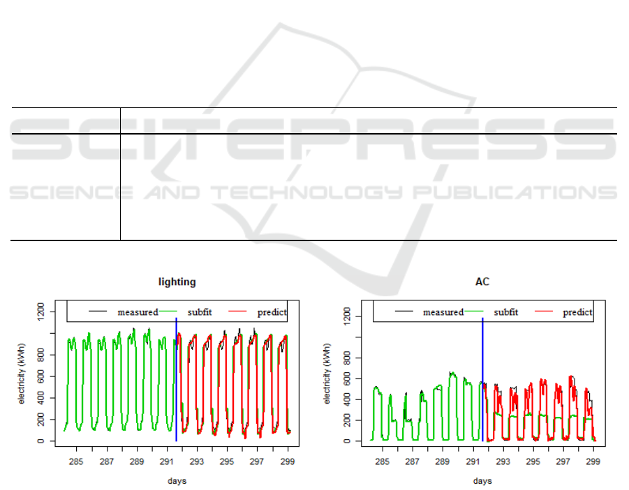
this item is much smaller than others, which hardly affects the total forecasting. Figure 2 compares

part of the measured and fitted values for the four types of appliances, and to be clearly, only results

of seven days before and after the boundary time of training and testing are shown. The figures show

that the model fits the measured values very well.

Table 1. Fit result for the training set, including the number of states (State No.), BIC, number

of degree of freedom, root mean square error (RMSE) and relative error.

State No.

BIC

NDF

RMSE

Relative error（%）

Lighting

66,844.81

447

15.02

1.98

Air condition

61,405.45

324

20.9

5.33

Movement

46,488.02

287

4.98

2.91

Management

46,416.37

447

3.41

15.25

Others

72,364.48

252

31.38

8.61

Aggregation

82,146.14

287

67.04

3.90

Forecasting Electricity Consumption of Appliances based on the Additive Factor Hidden Markov Model

197

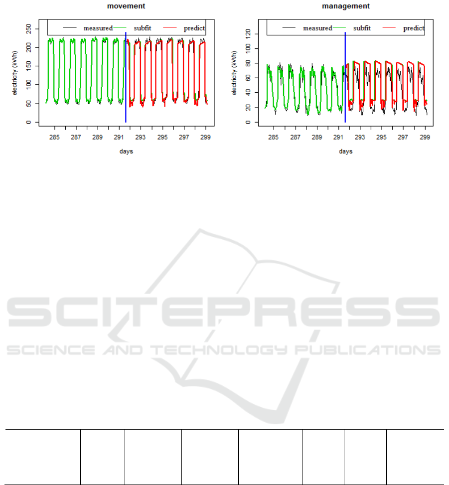
Figure 2. Comparison between the measured, model fit and forecasting values, where blue lines are

the boundaries for the training and testing sets, the black curves are measured values, the green

curves before the blue boundary lines are the model training results and after the blue lines are the

model forecasting values, and the red curves are adjusted values with aggregate data. The x-axis is

days, and the y-axis is electricity consumption.

3.2.2 Submodel forecasting in testing set. We predict the multi-stage for each appliance with an

optimized training model and influencing factors in the testing set and compare the expected values

with measured data in Table 2 and Figure 2. Table 2 lists the relative errors of prediction for all

appliances and the errors differ a lot for different appliances. Lighting and movement have the

smallest error, and their errors in training are also the smallest with lower than 3%. The air

conditioner has the largest forecasting error with 55.4% while its training error is not the largest,

meaning that the randomness of air conditioner usage is large, and the historical data cannot describe

all behaviors of air conditioners. For management and others, forecasting errors are 38.4% and 34.1%

and the training errors are also the largest, meaning that the model now has a limited ability to

describe the data. The comparison shows that the forecasting error is decided by both the

performance of training model and volatility of real electricity usage. Figure 2 also compares the

measured and forecasting values for each appliance in the testing part with the black and green

curves. To show the result clearly, only 180 hours in the training set and testing set are plotted.

Table 2. The relative error for model training, forecasting and adjustment processes.

Lighting

Air

conditioner

Movement

Management

Others

Mean

Aggregation

Training (%)

1.98

5.33

2.91

15.25

8.61

4.33

3.90

Forecasting (%)

13.99

55.39

12.52

38.32

34.10

21.51

16.33

Adjustment (%)

12.46

37.53

10.52

32.02

32.25

17.15

—

3.2.3 Adjusting the forecasting values with aggregate data. Combining the forecasting values of

appliances and aggregate electricity data in the testing set, the usage of appliances in the testing set

are adjusted and shown as red curves in Figure 2 and the relative errors are listed in Table 2. After

the adjustment of aggregate data, the estimated values of each appliance are closer to the real

measured values, especially for air conditioners. The relative errors of each appliance are also smaller

than simple model forecasting, especially for air conditioners and management such that the relative

error reduces from 55.4% and 38.4% to 37.6% and 32.1%. The mean relative error for all appliances

is only 17.15%, which corresponding to a very high accuracy.

IWEMSE 2018 - International Workshop on Environmental Management, Science and Engineering

198

3.3. Discussion

Above all, we get a result of mean accuracy 82.85% for the forecasting of appliances with hourly

data by using supervised AFHMM model, which is more accurate than other similar analyses.

Czarnek N. [16] compares the results for some public datasets with frequency of 1/s and 1/min by

several models, such as KNN, random forest, linear support vector machine and SVM with radial

kernel, where the accuracy ranges from 8% to 92%. Where only the accuracies of AMPds data

obtained by KNN and random forest models are larger than our work, but the data frequency is 1/min,

which is too large to be widely shared. Kolter J. Z [17] analyses the hourly Plugwise data with

supervised sparse coding model, but he only got a result with 55% accuracy. For the appliances,

lighting and movement have almost 90% accuracy, while for air conditioner and management, the

accuracy is only about 65% because of large fluctuation, meaning that we need improve the

performance of model with more attention on the usage of air conditioner and management. The

model in this work uses both data of appliances and aggregation for training, but in forecasting only

aggregation and influence factors data are used, which is possible to be applied in buildings without

appliance collectors only if we include the information of buildings in the training model.

4. Conclusions

In this paper, a supervised additive factorial hidden Markov model is developed by including

exogenous influences to forecast the electricity usage in appliance level. The model adopts EM

method to train the training dataset and obtain optimized parameters for submodel of each appliance

with both disaggregate and aggregate electricity data, and exogenous influence data. While in testing

process, the fitted parameters of submodels and exogenous influence data are used to forecast the

usage of appliances, and the aggregate electricity is used to adjust the values. The accuracy of the

model in training and testing dataset is calculated by comparing the estimated and measured values.

By applying the model to a dataset of one year hourly electricity consumption data for five types of

appliances in one building collected by smart meters in Shanghai, we get optimized parameters for

submodels with first 7,000 values as training set and forecast the appliances usage with last values as

testing set. The performance of model on training set is perfect with relative errors smaller than 7%

except for the usage of others. The performances of model in final forecasting results differ a lot for

different appliances, where the relative errors are 12.46%, 10.52%, 37.53%, 32.02%, 32.25% for the

usage of lighting, movement, air conditioner, management and others, respectively. The performance

of lighting and movement is best, while that of air conditioner is worst because of the large

randomness and fluctuation of usage in air conditioner for the diversity of human behaviors. We need

to pay more attention on the behaviour analysis on the usage of air conditioner to improve the

performance of model. The mean accuracy of all appliances is 82.85%, which is much higher than

analyses with same frequency data, and even larger than most analyses with higher frequency data.

The model proposed in this paper can forecast the usage of main appliances in hourly frequency

perfectly. In the future, we need to collect data of more types of buildings and include more influence

factors to extend the model and optimize the parameters of the model, in order to forecast the usage

of appliances for buildings without sub-collectors. The information about usage of appliances

feedback to users and energy suppliers can improve the efficiencies of energy-saving and monitoring,

which is a good way to overcome environmental pollution and shortages of resources.

Acknowledgment

This research is supported by the National 863 High Technology Research and Development Program of

China (2015AA050203) and the Science Project of State Grid Shanghai Municipal Electric Power

Company (52094016001Z).

References

[1] Kazandjieva and et al 2010 Technical Report CSTR 2010-03. Stanford University

Forecasting Electricity Consumption of Appliances based on the Additive Factor Hidden Markov Model

199

[2] Maile T 2010 Ph.D. Thesis. Department of Civil and Environmental Engineering, Stanford

University, CA.

[3] K Carrie Armel and et al 2013 Energy policy 52, 213-234

[4] Ehrhardt M and et.al 2010 Technical Reports E105, American Council for an Energy-Efficient

Economy, Washington, DC

[5] Gardner G T and Stern P C 2008 Science and Policy for a Sustainable Environment 50 (5),

12–24.

[6] Mercier C and Moorefield L 2011 Produced by ECOVA and Supported Through the California

Energy Commission’s Public Interest Energy Research Program

[7] Chirag D, Fan Z and et al 2017 Renewable and Sustainable Energy Reviews, 74 902-924

[8] Carlos A M and Mateus M G 2008 Electric Power Systems Research 78 721-727

[9] Cam M. Le, Daoud A and Zmeureanu R 2016 Energy 101 541-557

[10] Tao H, Pierre P and Shu F 2014 International journal of forecasting 30 357-363

[11] J Z Kolter and et al 2010 24th Annual Conference on Neural Information Processing Systems

[12] Kolter J Z and Jaakkola T 2012 The International Conference on Artificial Intelligence and

Statistics

[13] Yuan J H, Shen J K, Pan L and et al 2014 Renew Sustain Energy Rev 37(3) 896–906

[14] Schwarz and Gideon E1978 Annals of Statistics 6 (2): 461–464

[15] Shayle R and Searle 1982 Matrix Algebra Useful for Statistics. John Wiley and Sons

[16] Czarnek N, Morton K and Collins L 2015 IEEE international conference on smart grid

communications: Data management, grid analytics, and dynamic pricing

[17] Kolter J Z and Johnson M J 2011 SustKDD: San Diego, CA, USA

IWEMSE 2018 - International Workshop on Environmental Management, Science and Engineering

200