Segmentation Using Histogram and Fuzzy Entropy Principle

Jie Zhang

1,2

,Tao Han

,Hongli He

and Zanchao Wang

Institute of testing, Chinese Flight Test Establishment, Xi'an, China

School of Aviation, Beijing University of Areonautics and Astronautics, Beijing, China

Keywords: Fuzzy region, maximum fuzzy entropy principle, threshold, histogram, image segmentation.

Abstract: Segmentation of a composite image which contains two simple subimages is described. The a-priori

knowledge about the two simple subimages is that they possess the maximum amount of entropy. The

probability density functions(pdf s) of these image pixels are shown to be of theQuasi-gaussian form.

Parameters for the pdf are estimatedand then the maximum likelihood ratio test is applied to segmentation.

An iterative algorithm is employed to improve the segmentation accuracy. Extension of this method to the

segmentation of images with arbitrary pdf is discussed. This paper presents a thresholding approach by

performing fuzzy partition on a two-dimensional (2-D) histogram based on fuzzy relation and maximum

fuzzy entropy principle. The experiments with various gray level and color images have demonstrated that

the proposed approach outperforms the 2-D non-fuzzy approach and the one-dimensional(1-D) fuzzy

partitionapproach.

1 INTRODUCTION

The standard of evaluating the quality of the image

is mostly determined by the subjective of the

observer, and there is no general quantitative

criterion. Therefore, in the practical application of

image enhancement, several algorithms can be

selected for the specific application and several

enhancement algorithms. Then, how to select a kind

of algorithm with good visual effect and small

computation It comes out. To this end, only through

a number of representative image enhancement

algorithms in-depth, systematic study and

comparison, in order to find out their corresponding

advantages and disadvantages and the best

application scene, thus a set of effective application

of the image enhancement algorithm guidance rules.

Image enhancement techniques are used to

improve an image, where "improve" is sometimes

defined objectively (e.g., increase the signal-to-noise

ratio), and sometimes subjectively (e.g., make

certain features easier to see by modifying the colors

or intensities).

This section discusses these image enhancement

techniques:

 Intensity Adjustment

 Noise Removal

The functions described in this section apply

primarily to intensity images. However, some of

these functions can be applied to color images as

well. For information about how these functions

work with color images, see the reference pages for

the individual functions.

Simulation is a virtual representation of the

reality. It may also be defined as the process of

knowing the characteristics & exhibiting behavior of

a particular physical system. Sometimes a learner

finds it quite difficult to understand any physical

system behavior by just reading it from the written

material but once he is able to see the things actually

happening on the computer system the things really

change. That’s why the very important real life

techniques of image enhancement such as basic gray

level techniques, using arithmetic & logical

operations, using spatial filtering and also in the

frequency domain various filters like Low Pass

Filters, High Pass filters have been simulated on

Matlab and studied. The principal objective of

Enhancement a Images to process an Image so

suitable than the original image for a specific

application. Image Enhancement method falls into

two broad categories ways: Spatial Domain and

Frequency Domain methods.

Image segmentation in image processing and

image recognition system has a broad application

and prospects. Generally two different images have

different pdfs, and the work of determining the

difference is statistical in nature. The thresholding

method is a significant technique for image

processing and pattern recognition, which is

considered as the first step in image processing.

Many methods are proposed to select the automatic

threshold, while most of the single threshold

technology can be extended to multiple thresholds,

so this paper focuses on the single threshold. The

proposed method automatically determines the fuzzy

region and the threshold according to the maximum

entropy principle, thus to obtain the optimal solution

for the 2-D fuzzy entropy and the genetic

algorithm[1]. When the gray level is large, the

approximation is preferable, the standard deviation

is quite small and the average value is not at the

edge of the probability density function. This type of

images has been identified as images with the

maximum amount of entropy. According to the

research work above, these simple maximum

entropy images can be seen in many real life scenes,

such as television images.

2 THE PROPOSED METHOD

Complex images are composed of two simple image

pixels, the pixel value function is represented by

()

and

()

，and

is the pixel value. Thus,

the pdf of the Composite image is:

() () ( ) ()

1,01fx f x f x

ααα

=+− ≤≤

(1)

Where

is the mixing ratio and represents two

simple sub-images of the relevant type (measured by

the pixel). Although it is a point segmentation

method, but the overall consideration is also

feasible. Thus, only the gray value of the pixel is

used in the calculation of the image segmentation.

The largest possible inerratic classification for the

pixel

, so that the smallest possible error

must be satisfied.

()

≥−

(2)

In fact, when

and

()

are unknown to the

observer, then the pdf

()

of the composite image

is the only valid observation data. If the inequality is

estimated, then

and

()

must be predicted by

some practical methods

[2]

Define four adjacent mean

()

around pixel

()

()()

()

(, ) [ [ , 1 , 1

1, ( 1, )] 0.5]

xy f xy f xy f

fx y fx y

=++−++

++− +

(3)

The 2-D histogram is an array of

(, )

functions relative to the number of

occurrences. It can be seen as the two quantities

and

, where

is the gray level,

is the

average gray level, and

{

}

0,1, 2 1XY L== −L

The image points have the same intensity, but

different 2-D histogram of which different spatial

features may be distinguished in second dimensions

(local average gray level).

Block B and block W are each defined by (3),

and four fuzzy quantities

BrightX

DarkX

BrightY

, and

DarkY

are defined with the S

function and the corresponding Z function.

() ()

,,,

xX xX

BrightX x S x a b c

BrightX

∈∈

∑∑

(4)

() ()

,,,

xX xX

Dark x Z x a b c

DarkX

∈∈

∑∑

(5)

() ()

,,,

yY yY

BrightY y S y a b c

BrightY

∈∈

∑∑

(6)

() ()

,,,

yY yY

DarkY y Z y a b c

DarkY

∈∈

∑∑

(7)

Here,

()()

,,, 1 ,,,

xabc S xabc=−

.The fuzzy

relation Bright is a subset of the full analytic

space

XY×

, with

Bright BrightX BrightY X Y=×⊂×

(8)

() ()

()

min ,

Bright x y BrightX BrightY x y

rightX x BrightY y

μμ

=× =

(9)

Similarly, there are:

Dark DarkX DarkY X Y=×⊂×

(10)

()

() ()

()

(, ) ,

min ,

Dark x y DarkX DarkY x y

DarkX x DarkY y

μμ

=× =

(11)

Use the

()

function to define

as a fuzzy

set of elements

,1, ,

iN= L

()

is the

probability of occurrence of

. The maximum

entropy of the element

is defined by equation

(12)

[3]

() ()() ()

log

fuzzy A i i i

A xPx Px

=−

∑

(12)

The global entropy of the image is defined as:

()

()( )

image H Block H Block=+

(13)

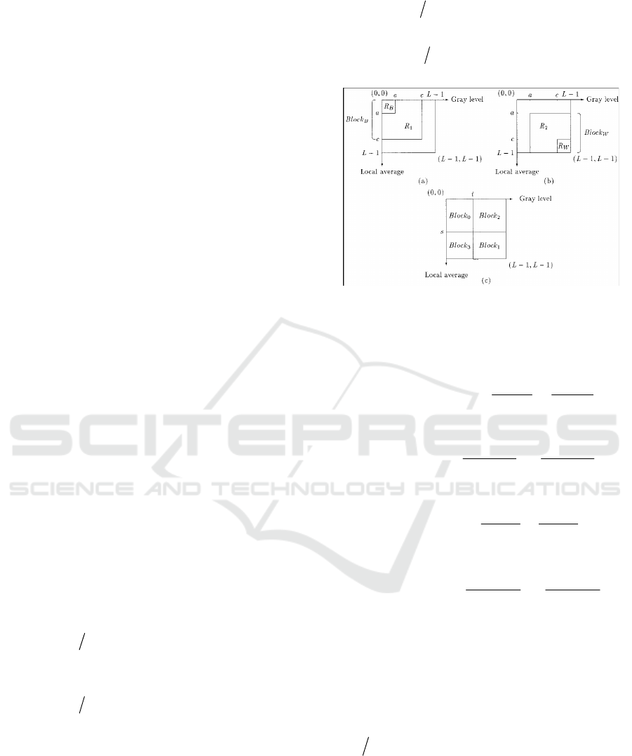
The dark block B as shown in Figure 1 can be

divided into a non-fuzzy region

and a fuzzy

region

1BB

lock R R=∪

(14)

() ()()

{

}

,,1,,

RxyDarkxy xyBlock

==∈

(15)

() ()()

{

}

,,1,,

RxyDarkxy xyBlock

=<∈(16)

Similarly, the bright block

Block

consists of a

non-fuzzy region

and a fuzzy region

, as

shown in Figure 1 (b).

1WW

lock R R=∪

(17)

() ()()

{

}

,,1,,

RxyDarkxyxyBlock

==∈

(18)

() ()()

{

}

,,1,,

RxyDarkxy xyBlock

=<∈

(19)

Figure 1: Image blocks.

The following four kinds of entropy can be

calculated as follows:

() ( )

()

,log

xy xy

fuzzy

xy R

yxy

xy R xy R

HR Darkxy

∈

∈∪

=−

∑

∑∑



(20)

()

log

xy xy

nonfuzzy B

xy R

yxy

xy R xy R

∈

∈∈

=−

∑

∑∑



(21)

() ( )

()

,log

xy xy

fuzzy

xy R

yxy

xy R xy R

HR Brightxy

∈

∈∈

=−

∑

∑∑



（22）

()

log

xy xy

nonfuzzy W

xy R

yxy

xy R xy R

∈

∈∈

=−

∑

∑∑



(23)

is the number of occurrences of

),( yx

the 2-D histogram. The membership

function

()

right x y

and

()

,Dark x y

are

defined by the equations (9) and (10), respectively.

It should be noted that the calculations

yxy

∑

in the four regions are independent.

3 IMAGE SEGMENTATION

PROCESS

Consider that the images are mixed by two

maximum entropy images

[4]

and both satisfy the pdf

that is the Gaussian distribution:

()

exp

2π

−

⎡⎤

=−

⎢⎥

⎣⎦

(24)

()

() exp

2π

⎡⎤

−

=−

⎢⎥

⎣⎦

(25)

In order to estimate

()

from the mixed pdf

s, some well-known classical measures such as

matrix method are applicable. One alternative is

to assume that

is 0 and

and

in the

mixed image

()

are constant in terms of

sample mean and sample deviations. The mixed

image contains a maximum entropy sub-image,

which is much smaller than the mixed image in

zize, for example,

is much less than 1%,

otherwise the probability of segmentation error

would be very large [5]. This iterative algorithm

will be discussed below, extended to the case of a

large

. The probability density curve is shown

in Figure 2.

Figure 2: Probability density.

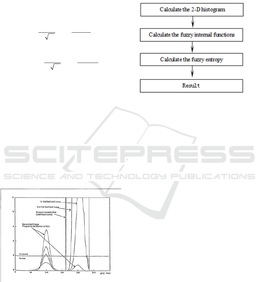
Finding the optimal a, b, c is an optimization

problem, which can be solved by heuristic search,

genetic algorithm

[6]

, stew fire simulation, etc. This

paper will use genetic algorithm to find the optimal

solution, and the process is shown in Figure 3. The

2-D histogram of the image is calculated first, then

the fuzzy internal functions on the 2-D histogram are

calculated, followed by the fuzzy entropy and finally

the result is obtained.

Figure 3: Optimal solution flow.

4 ANALYSIS OF RESULTS

Most grayscale horizontal image thresholding can be

extended to color images to directly process the

various components of the color space and then

combine the results to obtain the final image in one

way or another. Finally, process the color image in

each RGB color space respectively, and then merge

the three results to a new RGB color image

[7]

Therefore, a simulation system based on SUN

SPARC workstation is built to investigate the

performance of the iterative algorithm. For different

alternative image parameters, such as mean,

standard deviation and mixing ratio, this system will

be artificial synthesis. The iterations are then run on

the same machine and the iterative process is

investigated under different synthetic parameters

[8]

The simulation results show that if the segmentation

error is not large in the first run, then the pdf s of all

pixels is classified into different

()

Repeat this process to reduce the total classification

error until the end of the operation.

For Figure 4 (a), the threshold obtained by the 1-

D maximum fuzzy entropy method is 127, and the

entropy vectors obtained by the 2-D non-fuzzy

method and the 2-D fuzzy method are (119,159) and

(112,112) as shown in Figure 4 (b), Figure 4 (c) and

Figure 4 (d). Figure 4 (d) is clear than Figure 4 (b)

and Figure 4 (c) in detail, since the sky and the

tower are better segmented [9].

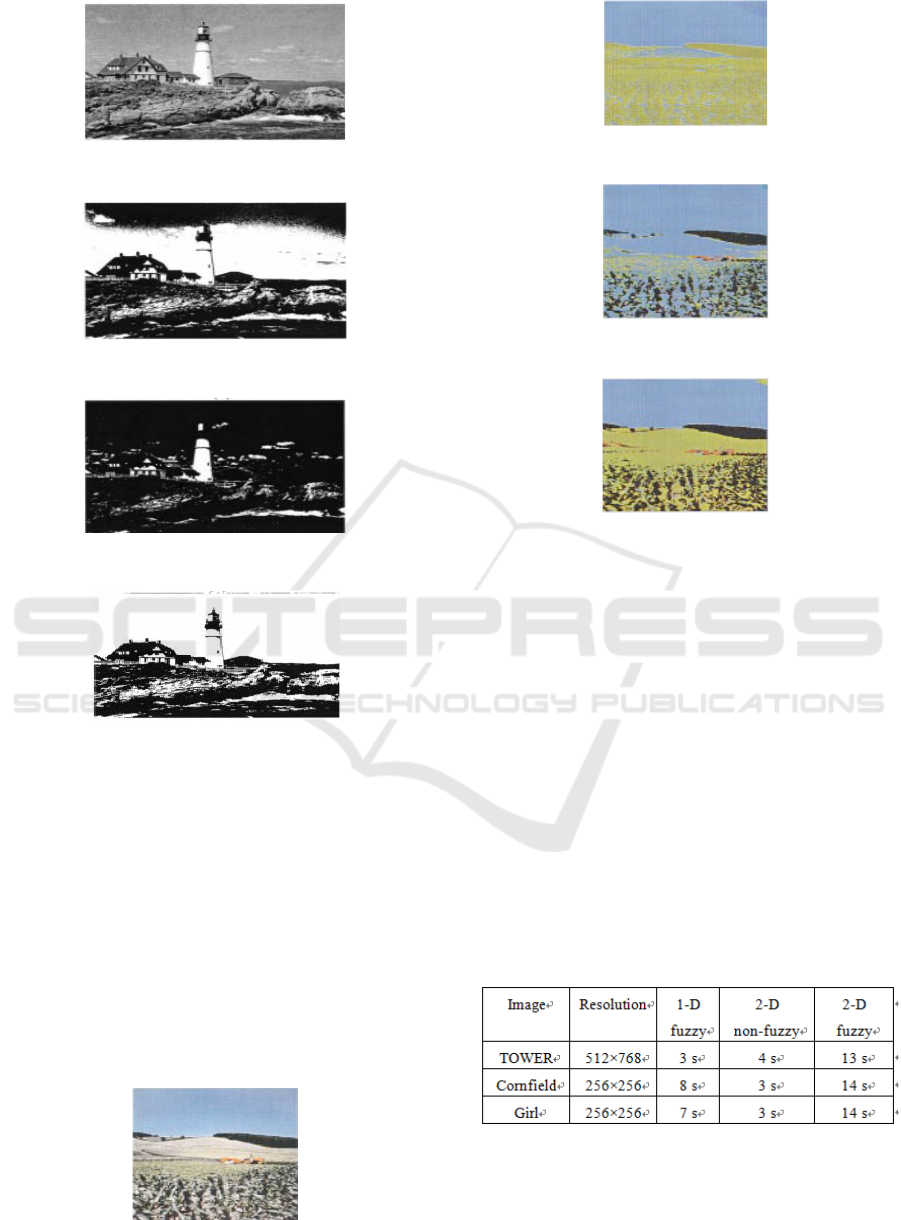
(a)

Original image

(b)

1-D fuzzy entropy result

(c)

2-D non-fuzzy entropy result

(d)

2-D fuzzy entropy result

Figure 4: Example 1 of image segmentation.

In Figure 5 (b), the three thresholds of RGB are

102, 113 and 112; for Figure 5 (c), the RGB

thresholds are (82, 82), (81, 75), and (66, 69); for

Figure 5 (d), the RGB threshold vectors are (81,81),

(100,100) and (154,154). Figure 5 (d) is the only one

that extracts the blue sky and the tractor from the

heaven and the earth, so the partition is better than

Figure 5 (b) and Figure 5 (c). The upper right corner

of Figure 5 (d) is misclassified because of the

threshold value which also appears in Figure 5 (c).

In summary, Figure 5 (d) gives the best results.

(a)

Original image

(b)

1-D fuzzy entropy result

(c)

2-D non-fuzzy entropy result

(d)

2-D fuzzy entropy result

Figure 5: Example 2 of image segmentation.

In Figure 6 (b), the RGB thresholds are 252, 211,

164; for Figure 6 (c), the threshold vectors are (138,

128), (164, 196), and (180, 182); for Figure 6 (d),

the threshold vectors are (215,215), (196,196),

(171,171). In Figure 6 (d), the eyes, nose and mouth

are extracted very well, the color of the clothes and

hair are also different. The color of the clothes, the

details of the hair and face are the same in Figure 6

(b). For Figure 6 (c), the clothes are misclassified to

the background, so they can not stand out of the

background

[10]

. This experiment is conducted on the

Lenovo G450 platform based on vc ++ 6.0, and the

computing time is shown in Table 1.

Table 1: Computing time.

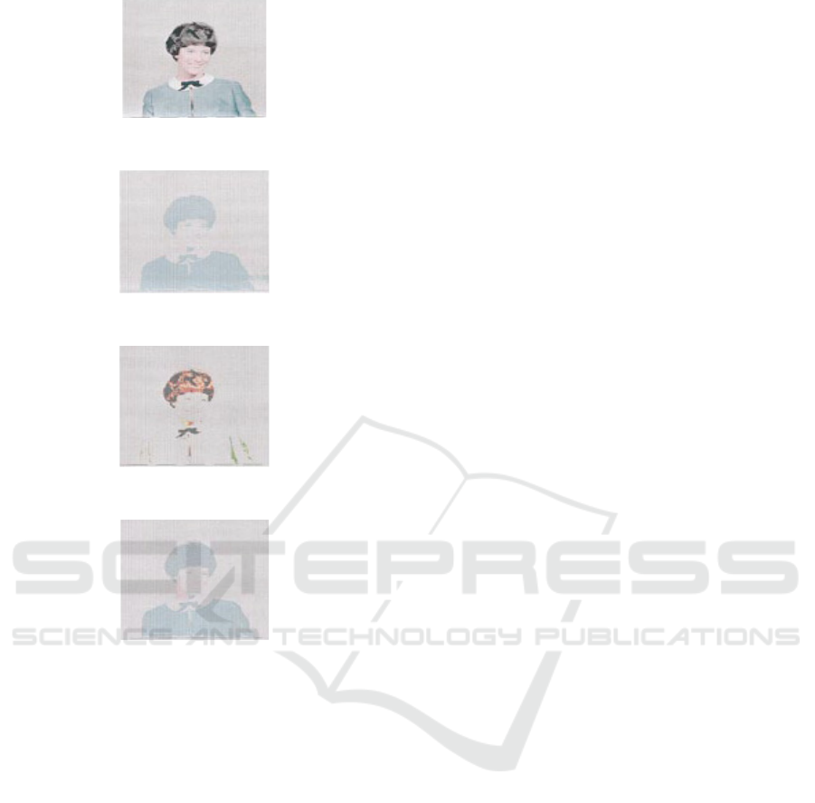
(a)

Original image

(b)

1-D fuzzy entropy result

(c)

2-D non-fuzzy entropy result

(d)

2-D fuzzy entropy result

Figure 6: Example 3 of image segmentation.

As can be seen from Table 1, the 2-D non-

fuzzy method outperforms the 1-D fuzzy and 2-

D fuzzy method in terms of computing time, and

the advantage is obvious.

5 CONCLUSIONS

In this paper, the parameters for the pdf s are

estimated first, and then the maximum likelihood

ratio test is applied to segmentation. The iterative

algorithm is employed to improve the accuracy of

segmentation and it is also extended to the

segmentation of images with arbitrary pdf s. The

experimental results indicate that the spatial

information of the pixels should be taken into

consideration when selecting the threshold, and the

2-D fuzzy approach is superior to the 2-D direct

maximum amount of entropy approach and 1-D

fuzzy entropy approach.

REFERENCES

1. Weiming, H., Tieniu T., 2004. A Survey on Visual

Surveillance of Object Motion and Behaviors, IEEE

Transactions on systems, man, and cybernetics.

2. Li He., Hui Wang., Hong Zhang., 2011. Object

Detection by Parts Using Appearance,Structural and

Shape Features. Mechatronics and

Automation(ICMA).

3. Anvaripour, M., Ebrahimnezhad, H., 2010. Object

Detection with Novel Shape Representation Using

Bounding Edge Fragments,Acta Photonica Sinica.

4. Wei, S., Baolong, G., Juanjuan, Z., 2010. Robust

Object Tracking via Hierarchical Particle Filter,

Telecommunications(IST).

5. Tingwu, Y., Zhengzhong, Z., 2014. Optical-Electronic

Measurement Theory and Methods in Flight Test,

National Defense Industry Publishing House,Beijing.

6. Comaniciu, D., Meer, P., 2002. Mean shift: a robust

application toward feature space analysis, IEEE

Transactions on Pattern Analysis and Machine

Intelligence.

7. Jian, X., Zhemin, D., 2005. Kalman Filter in Target

Tracking, Computer Simulation.

8. Nouar, O, D., Ali, G., Raphael, C., 2006. Improved

object tracking with Camshift algorithm, IEEE

International Conference onAcoustics.

9. Shiwei, G., Lei, G., Ning, Y., 2009. A New Particle

Filter Object Tracking Algorithm, Journal of Shanghai

Jiaotong University.

10. Lifeng, Q., Xinxi, F., Xiaoping, H., 2009. A New

Object Tracking Algorithm, Opto-Electronic

Engineering.