Lithology Identification by Support Vector Machine Using Well

Logging Data

ZhaojieZhang, Shi Fang

and WeiShen

College of Earth Science, Jilin University, Changchun 130061, China

Email: fs812625@vip.sina.com

Keywords: Lithology identification, support vector machine, genetic algorithm

Abstract: The Jurassic formation in the Fengcheng area of Junggar Basin has complicated lithofacies because of its

depositional environment supported the rapid deposition of sediment from a nearby provenance. The main

lithofacies of this formation are mudstone, fine-grained sandstone, medium-grained sandstone and

conglomeratic sandstone. Based on core and well logging data from the study area, this paper summarizes

the characteristics of the rock and analyzes the logging response characteristics of the lithology. We use

acoustic(AC), compensated neutron(CNL), density(DEN), gamma ray(GR) and resistivity(RT)logging data

as training and test samples to establish a lithofacies recognition model by using a support vector

machine(SVM). Additionally, we use a genetic algorithm to optimize the kernel parameter σ and penalty

factor C. The results show that the model predicts that the overall coincidence rate is 85.1%, which is better

than that predicted from a back-propagation(BP) neural network, and the model clearly improves the

lithofacies recognition accuracy and efficiency.

1 INTRODUCTION

The sandy conglomerate bodies of the Lower

Jurassic Badaowan Formation and Sangonghe

Formation in the Fengcheng area are mostly rapid

deposits, with features such as large vertical and

horizontal lithological changes, low compositional

maturity, and strong heterogeneity in various

lithologies (Bai et al., 2012). The logging response

characteristics are not significantly apparent in these

bodies. In the Fengcheng area, the formation

generally contains mud, ash, and pebbles,

representing a complex lithofacies formation that

complicates lithologic identification of the

conglomeratic sandstone (Liu et al., 2013).

However, considering the cost of the exploration

and development process, obtaining considerably

more core data is not possible and cutting logging

requires large sampling intervals. Therefore, it is

impossible to completely and accurately restore the

true lithology of the entire formation (Sebtosheikh et

al., 2015). Compared with core data, well logging

data are detailed, comprehensive and generally

continuous and are highly accurate in the

longitudinal direction, more comprehensively

reflecting the characteristics of the formation (Rider,

2002). So, in the field of lithology identification, it

is particularly important to determine the

interdependence of core data and logging data and to

integrate geological core data and logging data. At

present, conventional lithology identification

methods include several mathematical statistical

methods such as cross-plot methods (Fan et al.,

1999), principal component analysis, artificial neural

networks (Liu et al., 2007) and clustering methods

(Ghosh et al., 2016). However, the two-parameter

cross-plot method can effectively identify only the

well-characterized lithology from well logging data,

and it is difficult to recognize the lithology of an

entire well section or interpreted well section. When

we use the clustering method to identify lithology,

selecting different numbers of cluster centers has a

greater impact on the recognition accuracy. The

artificial neural network method is challenging

because of its network topology, and it is easy to fall

into a local minimum, resulting in a poor

performance of lithologic identification (Yu et al.,

2005). Although the principal component analysis

method can effectively reduce the logging data

dimensions and improve the recognition accuracy, it

is easy to ignore the well log attributes that have a

small value but have a great impact on the lithology

identification (Zhong and Li, 2009).

400

Zhang, Z., Fang, S. and Shen, W.

Lithology Identiﬁcation by Support Vector Machine Using Well Logging Data.

In Proceedings of the International Workshop on Environment and Geoscience (IWEG 2018), pages 400-405

ISBN: 978-989-758-342-1

Support vector machines is a machine learning

algorithm for both classification and regression

tasks. Based on the SVM method, the genetic

algorithm is used to optimize the parameters of the

SVM. In the case of limited core data, the logging

data are used to identify the lithology of the complex

conglomeratic sandstone in the Fengcheng area

(Mohammad and Ali, 2015; Mou et al., 2015). The

results of back-propagation (BP) neural network

prediction and SVM prediction are compared to

demonstrate the efficiency and feasibility of

lithography identification by using SVM.

2 METHODOLOGY

2.1 Support Vector Machine

SVM is a kind of machine learning method

developed on the basis of statistical learning theory.

SVM searches for the best trade-off between the

complexity and learning ability of the model

according to the limited sample information. SVM is

advantageous for solving problems with small

sample sizes, and nonlinear and high-dimensional

data recognition; additionally, SVM can find global

optimal solutions (Suykens and Vandewalle, 2000;

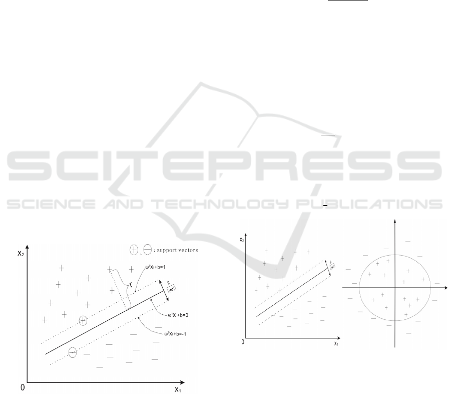
Vapnik, 1995). The main idea of SVM is to establish

a classification hyperplane as the decision-making

curve, which maximizes the isolation margin

between positive and negative examples (Gholam-

Norouzi et al., 2012). Its basic structure is shown in

Figure 1.

Figure 1: Support vectors and margin.

SVM evolves from the optimal separation

hyperplane in the case of linear separability. For a

second-class classification problem, given a training

data set on the feature space D={( 



,



) ，

(



,



),…,(



,



)}, where 



∈



,



∈



11



, i=1,2,…,N, N is the total number of

training samples and n is the dimension of the input

features. In sample spaces, the linear equation to

divide the hyperplanes is given as follows:



x+b=0 (1)

where ω is a normal vector that determines the

direction of the hyperplanes and b is a displacement

term that determines the distance between the origin

point and hyperplanes. Therefore, the distance

between any point (in the space) and the optimal

hyperplane can be written as follows:

r



xb



(2)

If the hyperplane can correctly separate training

samples, for(



,



)ϵ D, it satisfies Eqs(3).







b  1,



1;





b  1,



1.

(3)

Figure 1 shows several learning samples, and the

nearby hyperplanes are called “support vectors”.

The sum of the distances between the two

heterogeneous support vectors to the hyperplane are

satisfy Eq. (4).

γ=



‖‖

(4)

To move the positive and negative samples of

the training data set as far as possible from the

hyperplane, the maximum classification interval has

to satisfy Equation (5).

min





(5)



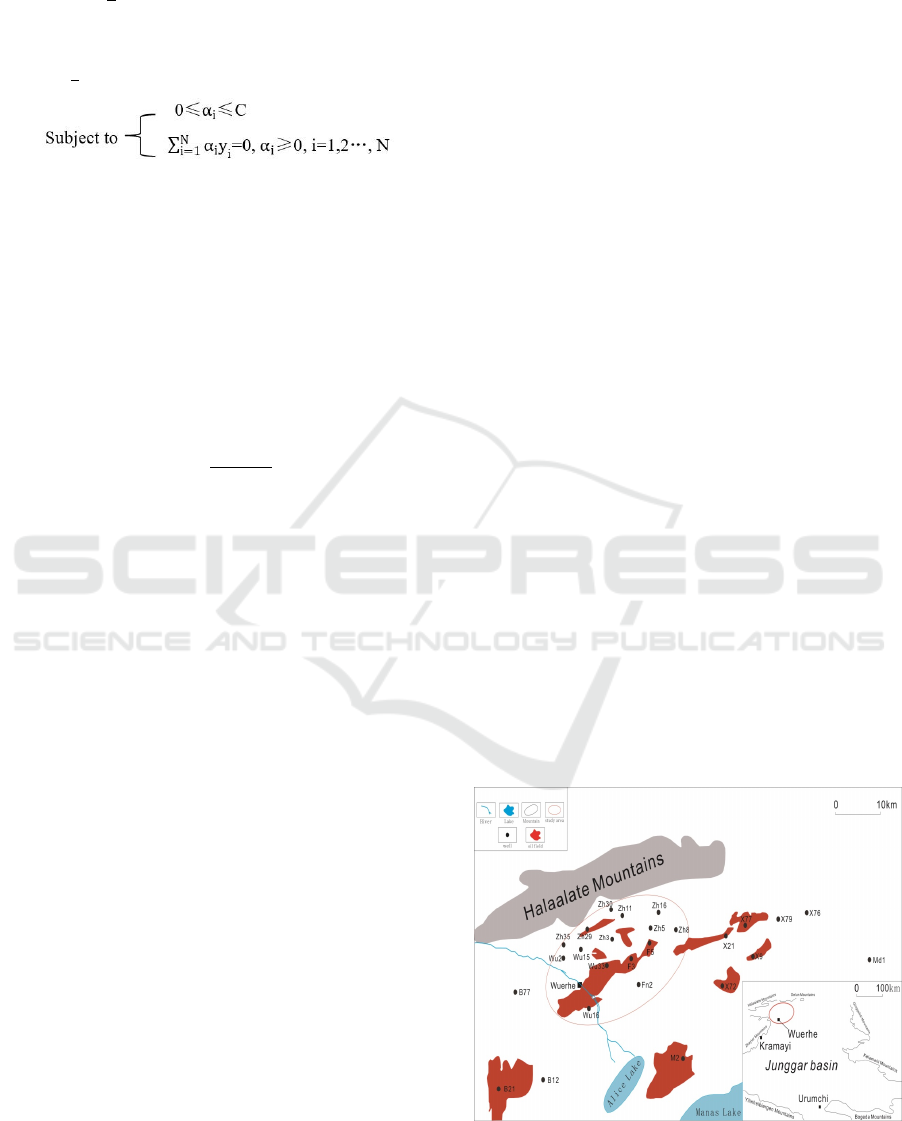
Figure 2: Two-category and Nonlinear classification.

In the nonlinear classification problem, no

hyperplanes in the original sample can correctly

classify the two types of samples (Figure 2) (Cheng

and Guo, 2010). For such a problem, we can add a

slack variable and a penalty factor into the SVM to

solve the problem, while using the Lagrange

multiplier method to transform the hyperplane

problem by dividing it into a dual problem. (Figure

2). This process satisfies Equation (6):

Lithology Identiﬁcation by Support Vector Machine Using Well Logging Data

401

L(w,b,α)=





‖w‖



∑







(w·x



+b)+

∑







(6)

where α



are Lagrange multipliers .() Equation

(6) can be changed into Equation (7):

min







∑∑



















·x



)-

∑







(7)



Solving the above equation to obtain the

classification decision function Eq.(8).

f (x)=

∑







k(x



，x



)+b (8)

This paper introduces the "kernel function"

method to solve the problem of nonlinear

classification. The original sample space data can be

transformed into a high-dimensional feature space

through nonlinear conversion to obtain the optimal

hyperplane. The most commonly used kernel

functions are the polynomial kernel, radial basis

kernel (RBF) and Sigmoid kernel. The RBF is used

as the kernel function in this paper.

K(



,



) = exp( -

‖







‖





) (9)

2.2 Genetic Algorithm

A genetic algorithm randomly searches for the

optimal solution, simulating the natural process of

evolution and the genetic mechanism in nature (De,

1975). It is a self-organizing and adaptive artificial

intelligence technology (Goldberg and Holland,

1988; Holland, 1975). The establishment of a SVM

model is essentially performed to identify two key

parameters: the kernel function parameter σ and

penalty factor C (Wu et al., 2009). The

determination of these two parameters has a great

influence on the accuracy and generalization ability

of this model. Here, we mainly introduce how to use

a genetic algorithm to realize the optimization of the

lithology recognition parameters of SVMs(Han et

al.,2012):

Input standardized lithology samples as training

samples.

Randomly generate a set of SVM parameters,

each parameter is encoded by using a binary coding

scheme to construct an initial population.

Calculate the cost function to determine fitness,

A greater cost function result indicates a lower

fitness.

Select a number of individuals with high fitness,

and determine the next generation with direct

genetic.

Using the crossover, mutation and other genetic

operators to address the current generation of

groups, generate the next generation of groups.

Repeat step b, evolving a set of initially

determined SVM parameters until the training

objective satisfies the condition.

3 DATA PREPARATION

The Fengcheng area is located in the northwestern

part of the Junggar Basin (Figure 3). The strata in

the basin are thin in the north but thick in the south,

creating wedge shape that thickens into the basin.

Among the formations in the basin, the Lower

Jurassic Badaowan Formation is dominated by

braided river deposits and developed lithologies

such as mudstone, siltstone, fine-grained sandstone,

medium-grained sandstone and conglomeratic

sandstone (Wang et al., 2012). The Sangonghe

Formation is generally composed of braided river-

delta deposits. The lithologies of the Sangonghe

Formation are mudstone, silty mudstone, siltstone,

fine-grained sandstone, medium to coarse-grained

sandstone and conglomeratic sandstone (Zhu et al.,

2017). This paper combines the lithologies and

logging data and takes the Jurassic formation as an

example, analyzing the logging response

characteristics under different lithologies, and

extracting the logging response parameters that are

sensitive to lithology to establish a GA-SVM

lithology model, to study a method for the

conglomeratic sandstone lithology identification and

its application (Feng et al., 2002).

Figure 3: The location of study area.

IWEG 2018 - International Workshop on Environment and Geoscience

402

Due to the complexity of the lithology in the

study area, four major lithologies were identified

based on the available data: mudstone, fine-grained

sandstone, medium-grained sandstone and

conglomeratic sandstone. In this paper, 274

representative lithological samples were selected

from 20 wells with accurate core identification data

in the study area. The samples included 75

mudstone, 62 fine-grained sandstone, 47 medium-

grained sandstone, 90 conglomeratic sandstone

samples. We extract density (DEN), neutron

porosity (CNL), acoustic (AC), true formation

resistivity (Rt), and gamma ray (GR) response

characteristics from conventional logging data to

establish a sample space of 5 dimensions and 4

types. Table 1 shows the logging response

characteristics of four lithologies in the study area.

Table 1 shows that many differences exist among

the different logging parameters for each lithology

and provides the initial conditions for the lithology

identification. Additionally, to eliminate the

influence of the different dimension of the features,

the logging parameters of the samples were

normalized and uniformly included in the range of

(0,1).

Table 1: Logging response of sandy conglomerate in Fengcheng area.

lithology

AC/(μs·m



)

CNL/(%)

DEN/(g·cm



)

GR/(API)

RXO/(Ω·m)

Logging response

mudstone 108~145 30~42 1.7~2.2 74~104 4~9 low RXO medium-low DEN

Fine-grained sandstone 112~129 29~41 2.0~2.2 50~78 21~96 low GR medium-high RXO

medium-grained sandstone 104~117 29~36 2.0~2.3 55~67 13~28 low RXO low GR

conglomeratic sandstone 65~110 18~31 2.1~2.4 56~103 36~91 low AC low CNL high RXO

Table 2: Learning samples.

Depth/m

(μs·m



)

CNL

(%)

DEN(g·cm



)

(API)

RXO(Ω·m)

lithology

386 120.0022 33.14312 2.245676 85.88315 7.251

439 131.3215 34.71169 2.256805 101.3727 4.984

440 120.5571 32.04662 2.29659 92.85284 9.829

462 129.7608 38.39526 2.176265 93.98495 4.984

252 134.9082 32.97143 2.265457 92.06599 4.305

661 110.3771 29.9864 2.245051 56.77773 38.888

628 94.20476 31.01351 2.244652 69.63533 45.213

621 100.1302 28.73366 2.228544 61.22003 66.728

392 104.1054 29.8592 2.22488 65.2195 49.2

426 89.4013 29.24075 2.28078 81.11826 39.253

391 115.2215 29.44463 2.193363 67.0258 24.766

534 129.3597 40.09695 2.143977 71.84998 68.099

619 127.3185 33.00572 2.105721 55.42553 52.74

352 127.3506 33.68263 2.104538 72.79697 23.696

354 125.9028 33.70022 2.083479 77.45229 26.639

638 107.1057 29.46306 2.247549 58.19688 15.851

639 101.8406 36.56046 2.260366 58.03394 19.848

632 107.1129 32.45584 2.244591 55.58301 28.541

636 108.4648 33.97344 2.210082 63.91458 18.279

606 116.9149 32.27015 2.152229 64.24762 16.201

Notes: 1- mudstone;2- conglomeratic sandstone;3- Fine-grained sandstone; 4- medium-grained sandstone

Lithology Identiﬁcation by Support Vector Machine Using Well Logging Data

403

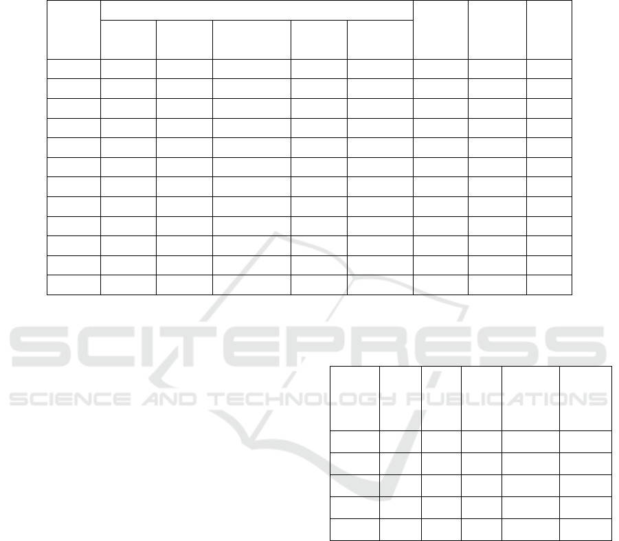
Table 3: Test samples.

Depth/m

Logging response

lithology

actual

GA-SVM

predict

BPNN

predict

(μs·m



)

CNL

(%)

DEN(g·cm



)

(API)

RXO(Ω·m)

465

147.3778 34.18616 2.169473 90.90363 7.037

1 1 1

351

108.135 33.05614 2.24345 75.90002 7.415

1 2 3

352

117.9064 34.04599 2.253468 91.61892 8.069

1 1 2

386

121.4397 33.79903 2.221189 87.09536 7.416

1 1 1

428

69.20372 18.59011 2.404825 102.4146 67.4

2 2 2

426

72.99623 18.92969 2.369991 96.1902 57.358

2 2 1

358

125.9543 35.29397 2.103536 76.91651 25.319

3 3 4

350

127.6563 34.53033 2.066431 70.86774 20.841

3 3 3

606

117.9348 34.07982 2.171098 73.35375 14.199

4 4 4

634

116.7718 33.65931 2.160615 78.34065 18.599

4 3 1

604

104.3699 33.76941 2.263324 61.09675 18.379

4 4 2

608

109.3916 33.06219 2.285016 73.96328 18.728

4 2 4

4 RESULTS AND DISCUSSION

The quality of the SVM classification largely

depends on the choice of the parameter σ and

penalty factor C of the kernel function. Choosing

unreasonable parameters will directly affect the

prediction accuracy. Therefore, in this paper, based

on the selection of a radial basis kernel function as

the kernel function used by the SVM, the optimal

parameter value (23.679, 4.4169) is calculated by

the genetic algorithm.

After obtaining the optimized kernel function

parameter σ and penalty factor C, 200 lithologic

samples are trained as learning sets (Table 2) to

obtain a corresponding SVM model, while 74

lithologic samples are used as test sets to test the

lithologic identification model, the results of which

are compared with the BP neural network method.

Table 3 lists the input parameters and identification

results of some of the test samples. Table 4 shows

the classification of all the test samples.

Table 3 and Table 4 show that the GA-SVM

method provides good lithologic identification

results. Compared with the BP neural network

model, which trained with the same samples, the

accuracy of the GA-SVM result is higher. The GA-

SVM method correctly identified 63 samples from

all the test samples, for an accuracy rate of 85.1%,

while the identification accuracy of the BP neural

network was only 60.8%.

Table 4: Accuracy of SVM lithology identification.

Lithologysamples GA-

SVM

BPNN GA-SVM

accuracy

BPNN

accuracy

1 15 12 10 80 66.6

2 22 18 13 81.8 59

3 20 19 14 95 70

4 17 14 8 82.3 47

total 74 63 45 85.1 60.8

5 CONCLUSIONS

The formation environment of conglomeratic

sandstone is complex: major structural and

compositional changes occur, and the heterogeneity

is strong. This environment creates challenges for

the identification conglomeratic sandstone lithology.

To reduce the multiplicity of corresponding relations

between logging responses and lithologiesy, we

identify the correlation between conventional

logging data and the lithology of a conglomeratic

sandstone.

IWEG 2018 - International Workshop on Environment and Geoscience

404

By using the classification advantage of support

vector machines for nonlinear problems with small

samples sizes, we can precisely categorize the

lithology of the conglomeratic sandstone .

The genetic algorithm can effectively search for

the optimal parameters of support vector machines.

Using the genetic algorithm to build the support

vector machine lithology identification model, the

overall prediction rate of the test samples is 85.1%,

which is better than that using the BP neural

network.

ACKNOWLEDGMENTS

This work was supported by the National Natural

Science Foundation of China under Grant

Nos.41472173.

REFERENCES

Bai Y, Xue L F and Pan B Z 2012 Multi-Methods

Combined Identify Lithology of Glutenite Journal of

Jilin University (Earth Science Edition)(in Chinese)

42(sup2) 442-451

Cheng Guo-jian and Guo Rui-hua 2010 Application of

PSO-LSSVM classification model in logging lithology

recognition Journal of Xi'an Shiyou University(Natural

Science) 01 96-99

De Jong K A 1975 Analysis of the behavior of a calss of

genetic adaptive systems. Ann Arbor: The University

of Michigan Press

Fan Y R, Huang L J and Dai S H 1999 Application of

crossplot technique to the determination of lithology

composition and fracture identification of igneous rock

Well Logging Technology. (in Chinese) 23(1) 53-56

Feng G Q, Chen J and Zhang L H 2002 Realizing Genetic

Algorithm of Optimal Log Interpretation Natural Gas

Industry(in Chinese) 22(6) 48-51

Gholam-Norouzi , Abbas Bahroudi and Maysam Abedi

2012 Support vector machine for multi-classification of

mineral prospectivity areas Computers & Geosciences

46 272-283

Ghosh S, Chatterjee R and Shanker P 2016 Estimation of

Ash, Moisture Content and Detection of Coal

Lithofacies from Well logs using Regression and

Artificial Neural Network Modelling Fuel 177 279-287

Goldberg D E and Holland J H 1988 Genetic algorithms

and machine learning Machine Learning 3(2) 95-99

Han X, Pan B Z and Zhang Y 2012 GA-Optimal Log

Interpretation Applied in Glutenite Reservoir

Evaluation Well Logging Technology (in Chinese)

36(4) 392-396

Holland J H 1975 Adaptation in natural and artificial

systems.Ann Arbor:The University of Michigan Press

Liu Q R, Xue L F and Pan B Z 2013 Study on Glutenite

Reservoir lithology Identification in Lishu Fault Well

Logging Technology. (in Chinese) 37(3) 269-273

Liu X J, Chen C and Zeng C 2007 Multivariate statistical

method of utilizing logging data to lithologic

recognition Geological Science and Technology

Information. (in Chinese) 26(3) 109-112

Mohammad Ali Sebtosheikh and Ali Salehi 2015

Lithology prediction by support vector classifiers using

inverted seismic attributes data and petrophysical logs

as a new approach and investigation of training data set

size effect on its performance in a heterogeneous

carbonate reservoir Journal of Petroleum Science and

Engineering 134 143-149

Mou Dan , Wang Zhu-Wen and Huang Yu-Long 2015

Lithological identification of volcanic rocks from SVM

well logging data : Case study in the eastern depression

of Liaohe Basin Chinese J.Geophys. (in Chinese) 58(5)

1785-1793

Rider M 2002 The geological interpretation of well logs ,

2nd edn. Rider-French Consulting Ltd ., Sutherland

Sebtosheikh M A, Motafakkerfard R and Riahi M A 2015

Support vector machine method, a new technique for

lithology prediction in an Iranian heterogeneous

carbonate reservoir using petrophysical well logs

Carbonates and Evaporites 46 272-283

Suykens J A K and Vandewalle J 2000 Recurrent least

squares support vector machines IEEE Transactions on

circuits and System-I 47(7) 1109-1114

Vapnik V 1995 The Nature of Statistical Learning Theory.

Springer-Verlag, New York

Wang Y, Peng J and Zhao R 2012 Dentative Discussions

on Depositional Facies Model of Braided Stream in the

Northwestern Margin, Junggar Basin: A case of

braided stream deposition of Badaowan Formation,

Lower Jurassic in No.7 Area Acta Sedimentologica

Sinica (in Chinese) 30(2) 264-273

Wu Jing-Long , Yang Shu-Xia and Liu Cheng-Shui 2009

Parameter selection for support vector machines based

on genetic algorithms to short-term power load

forecasting Journal of Central South

University(Science and Technology) (in Chinese) 40(1)

180-184

Yu D G, Sun J M and Wang H Z 2005 A New Method for

Logging Lithology Identification – SVM Petroleum

Geology & Oilfield Development in Daqing. (in

Chinese) 05 93-95

Zhong Y H and Li R 2009 Application of principal

component analysis and least square support machine

to lithology identification Well logging Technol (in

Chinese) 33 425-9

Zhu X M, Li S L and Wu D 2017 Sedimentary

characteristics of shallow-water braided delta of the

Jurassic, junggar basin, Western China Journal of

Petroleum Science and Engineering 149 591-602

Lithology Identiﬁcation by Support Vector Machine Using Well Logging Data

405