A Cone Loaded Ultra-Broad Band Antenna
For Electric-Field Measurement
Ziqian Zeng and Hongfu Guo
School of Physics and Optoelectronic Engineering, Xidian University, Xi’an, Shaanxi, China
Keywords: Electric-field probe, Tapered antenna, Cone dipole, Loading, Ultra-broad band.
Abstract: The design of sensing antennas in electric-field probes is the key to measure electromagnetic radiation
accurately. In this paper, the cone dipole antenna and its dimension parameters are simulated by Ansoft
HFSS. Meanwhile, the impact of dimension parameters on the performance of antennas is analysed. In order
to improve the flatness of probe, the loaded dipole is adopted. Combining with the detection characteristics
of diodes, the relationship between performance of loaded antennas and the flatness of electronic-field
probes is discussed. Finally, the 1-40GHz ultra-broad band antenna for electric-field measurement is
developed by optimizing these parameters of the antenna.
1 INTRODUCTION
The electromagnetic waves has provided unlimited
convenience for people’s lives. However, the
problem caused by electromagnetic radiation is also
highlighted gradually. Now electromagnetic
radiation has risen to a new source of pollution, the
electromagnetic pollution (Hou, 2011).
Electromagnetic environment monitoring is an
extremely effective way to reduce the harm caused
by electromagnetic radiation to human. And electric-
field probe is the core component of electromagnetic
environment monitoring (Li, 2016).
In recent years, many experts have developed
various electric-field probes and sensing antennas.
Lv (2014) developed a broadband electric-field
probe based on the fractal structure which improved
the low frequency response of an ordinary electric-
field probe, composed by the straight dipole. Then,
Togo (2014) developed a metal-free electric-field
probe based on photonics. Its frequency response is
flat within a 6 dB range at frequencies from 100kHz
to 10GHz. Later, Ohoka et al. (2015) developed an
electric-field probe that combined a small dipole
antenna with a high input impedance differential
input amplifier circuit. This probe significantly
improved sensitivity at low frequency. Nevertheless,
now because the frequency needed by electronic
systems becomes increasingly high and the upper
limit of frequency range is already more than
40GHz, the existing antennas in electric-field probes
no longer apply it. The antenna is the
main component
of the probe (Harasztosi, 2002). Therefore, the design
of ultra-broad band sensing antennas in electric-field
probes becomes the crux of the design of electric-
field probes (Sun, 2008).
Based on the characteristic of antennas that the
conventional dipole antenna is highly frequency
sensitive (Kanda and Driver, 1987), the tapered
structure and the loaded dipole have been used to
solve above problem. In this paper, cone loaded
dipole antennas are simulated and the impact of its
parameters on the frequency response is analysed.
Finally, the cone loaded ultra-broad band dipole
antenna which the useful frequency range is up to 1-
40GHz is realized by optimizing parameters.
2 DESIGN CONSIDERATIONS
FOR THE ANTENNA IN THE
ELECTRIC-FIELD PROBE
The electric-field probe consists of an electrically
short dipole antenna and detector diode connected to
an instrumentation amplifier via a high impedance
line (Kalyanasundaram and Arunachalam, 2011).
The performance of electric-field probes is mainly
influenced by both the receiving antenna and the
detector diode. The detection characteristic of ideal
diode circuits is non-linear that the higher the
Zeng, Z. and Guo, H.
A Cone Loaded Ultra-Broad Band Antenna For Electric-Field Measurement.
In 3rd International Conference on Electromechanical Control Technology and Transportation (ICECTT 2018), pages 455-459
ISBN: 978-989-758-312-4
Copyright © 2018 by SCITEPRESS – Science and Technology Publications, Lda. All rights reserved
455

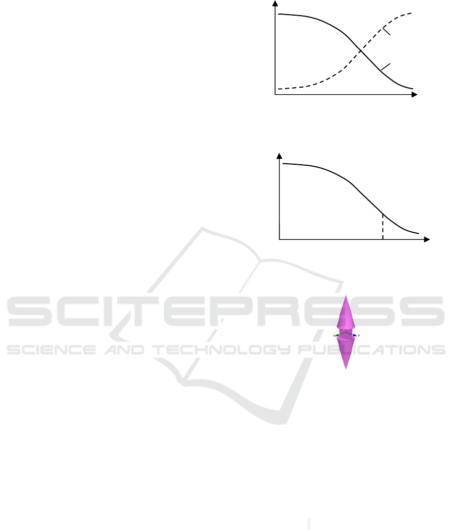
frequency is, the worse the performance of the
detected output is, as shown in Fig. 1. Therefore, to
attain an electric-field probe with flat frequency
response, the efficiency of the receiving antenna and
the detector diode should be complementary that the
performance of the receiving antenna increases with
increasing frequency, as shown in Fig. 1. If using
reflection coefficient (S11) to discuss the
performance of the antenna, S11 should decrease
with increasing frequency, as shown in Fig. 2.
In the paper, we want to attain an ultra-broad
band antenna with useful frequency range of 1-
40GHz. Therefore, the efficiency of the antenna
should increase with increasing frequency within the
frequency range of 1-40GHz.
3 SIMULATION FOR ANTENNAS
IN THE PROBE
According to the antenna theory, the relationship
between the frequency and reflection coefficient
(S11) of the tapered antenna is similar to the one we
need. In practical engineering applications, there are
different kinds of tapered antennas, such as cone
dipole antennas, pyramid dipole antennas and so on.
In the paper, the cone dipole antenna is selected
because it’s easy to process. In order to facilitate
simulate and design, the cone unloaded antenna is
simulated first, and the relationship between the
frequency and its parameters is analysed. Then by
simulating the loaded antenna and optimizing
parameters, the optimal parameters is obtained.
3.1 Simulation and Design for the
Unloaded Dipole Antenna
Fig. 3 shows the simulation model of cone dipole
antenna whose material is copper. The performance
of antennas is analysed by changing its parameters.
Final, the optimal antenna is obtained.
3.1.1 The Impact of Antenna Length on the
Antenna Performance
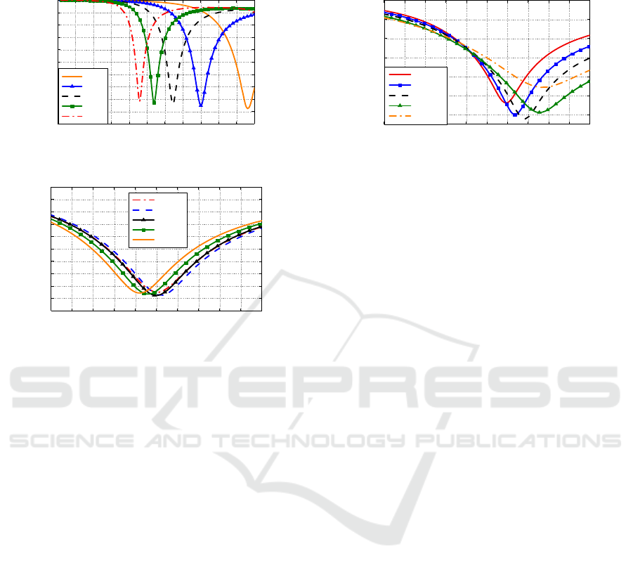
In the simulation, the antenna length is changed
from 3mm to 8mm and the step size is 1mm. Besides,
the cone radius of the dipole and the dipole gap are
set as 0.1mm and 0.5mm respectively. The
simulation results shown in Fig. 4 indicates that the
impact of the antenna length on resonant frequency
is obvious. It can be observed that resonant
frequency decreases with increasing antenna length.
Figure 1: The efficiency of detected circuit and receiving
antenna.
Figure 2: S11 versus frequency in the receiving antenna.
Figure 3: Cone dipole antenna model.
Besides, the 4-mm dipole antenna whose
resonant frequency is 40GHz meets the requirement
that the efficiency of the antenna should increase
with increasing frequency within the range of 1-
40GHz.
3.1.2 The Impact of the Dipole Gap on the
Antenna Performance
Based on the above length optimization, the length is
set as 4mm. And the dipole gap ranges from 0.1mm
to 1mm and the step size is 0.1mm. Besides, the
cone radius of the dipole is set as0.1mm. Figure 5
shows that the dipole gap has slight influence on
antenna performance. When the dipole gap is 0.7mm,
the efficiency around 40GHz is highest.
Freq.
Detected output/ fre
q
uenc
y
res
p
onse
Receiving antenna
Detector circuit
S11
(
dB
)
40GHz
Fre
q
.
ICECTT 2018 - 3rd International Conference on Electromechanical Control Technology and Transportation
456

3.1.3 The Impact of Cone Radius on the
Antenna Performance
0 5 10 15 20 25 30 35 40 45 50 55
-20
-18
-16
-14
-12
-10
-8
-6
-4
-2
0
S11 (dB)
Freq. (GHz)
3mm
4mm
5mm
6mm
7mm
Figure 4: S11 versus frequency for varying antenna length.
35 36 37 38 39 40 41 42 43 44 45
-20
-18
-16
-14
-12
-10
-8
-6
-4
-2
0
S11 (dB)
Freq. (GHz)
0.5mm
0.6mm
0.7mm
0.8mm
0.9mm
Figure 5: S11 versus frequency for varying dipole gap.
Here the antenna length and the dipole gap are
set as 4mm and 0.7mm respectively. And the cone
radius of the dipole is changed from 0.1mm to
0.7mm. In Fig. 6, with cone radius increasing,
reflection coefficient (S11) of resonant frequency
point decreases first and then increases. When the
cone radius of the dipole is 0.5mm, the efficiency of
the antenna is highest.
According to above simulation, when antenna
length, the dipole gap and cone radius are 4mm,
0.7mm and 0.5mm respectively, the performance of
antenna is best. However, compared with ideal
antenna shown in Fig. 2, the performance of above
antenna has huge difference from the one we need.
Its resonant characteristic is too prominent.
3.2 Simulation and Design for loaded
Dipole Antennas
According to antenna theory and above analysis, the
bandwidth of the dipole with pure metal is very
narrow. Its resonant characteristic is prominent.
While loaded antennas have flatter frequency
response and wider bandwidth. Therefore, loaded
antennas are used to improve the performance of
antennas in probes (Yang et al., 2014).
In last section we know that the impact of
antenna length on resonant frequency is obvious, so
the length and the loaded surface resistance are
mainly changed to optimize the performance of
antennas in this section. Here the dipole gap and
30 32 34 36 38 40 42 44 46 48 50
-24
-20
-16
-12
-8
-4
0
S11 (dB)
Freq. (GHz)
0.3mm
0.4mm
0.5mm
0.6mm
0.7mm
Figure 6: S11 versus frequency for varying cone radius.
cone radius are set as the optimal results which are
0.7mm and 0.5mm, and the substrate material of
dipoles is aluminium-oxide (Al
2
O
3
). In the loaded
antenna design, the resistance and the excitation
probably have poor contact when the dielectric and
the excitation are directly connected. So a sheet
metal (gold) with 0.1-mm thickness is added
between the dielectric and the excitation.
3.2.1 Optimization for Antenna Length
First, we optimize the length of loaded antenna. In
the process, based on that free space intrinsic
impedance is 377Ω, the surface resistance of single
arm of the dipole is set as 400Ω (Kraus, 2011).
Meanwhile, antenna length is changed from 3mm to
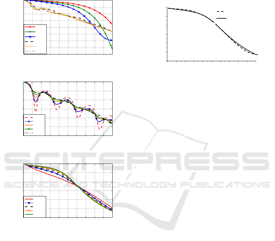
30mm. From the simulation results in Fig. 7, we can
know that short loaded antennas have low efficiency,
especially in the range of 1-30GHz. Then, the
efficiency becomes high and the flatness becomes
good by increasing antenna length. And the 25mm
loaded dipole antenna has the best performance.
3.2.2 Optimization for Surface Resistance
In order to obtain the optimal loaded antenna, the
surface resistance is changed in this section.
Antenna length is set as optimal value, 25mm. Fig. 8
depict the frequency response with different
resistance. First, we change the resistance around
400Ω, as shown in Fig. 8(a). It can be seen that there
are several resonance points within 1-40GHz, and
resonance characteristic becomes weak by
increasing resistance. Then, we continue to increase
resistance. Fig. 8(b) shows that the efficiency
becomes low within the range of 1-30GHz and
becomes high within the range of 30-40GHz when
the resistance increases. And now the trend of S11
curves is close to the ideal antenna.
A Cone Loaded Ultra-Broad Band Antenna For Electric-Field Measurement
457

By simulating unloaded and loaded antennas, we
obtain the optimal antenna whose size is 25-mm
antenna length, 0.7-mm dipole gap and 0.5-mm cone
radius. And when the surface resistance is 4000Ω, its
0 5 10 15 20 25 30 35 40 45 50
-16
-14
-12
-10
-8
-6
-4
-2
0
S11 (dB)
Freq.(GHz)
3mm
4mm
5mm
20mm
25mm
30mm
Figure 7: S11 versus frequency for varying antenna length.
0 5 10 15 20 25 30 35 40 45 50
-12
-10
-8
-6
-4
-2
0
S11 (dB)
Freq. (GHz)
100Ω
200Ω
300Ω
400Ω
500Ω
(a)
0 5 10 15 20 25 30 35 40 45 50
-12
-10
-8
-6
-4
-2
0
S11 (dB)
Freq.(GHz)
1000Ω
2000Ω
3000Ω
4000Ω
5000Ω
(b)
Figure 8: (a) S11 versus frequency for resistance of 100-
500Ω. (b) S11 versus frequency for resistance of 1000-
5000Ω.
performance is closest to our need. Compared with
the ideal antenna, the frequency response of the
above optimal antenna can fit it well, as shown in
Fig. 9. So it can be used in the probe.
4 CONCLUSIONS
In the paper, we analyse cone unloaded and loaded
antennas. The results indicate: 1) Loading resistance
has a great influence on S11 curve of the antenna. 2)
Loading resistance can obviously improve the
flatness of the antenna in electric-field probe.
In this work, the broad-band antenna in probes for
electric-field measurement with working frequency
of 1-40GHz is presented by using cone structure and
0 5 10 15 20 25 30 35 40 45 50
-12
-10
-8
-6
-4
-2
0
S11 (dB)
Freq (GHz)
Figure 9: The comparison of ideal and simulated antenna.
loaded dipole. And the method in the paper can be
used to design antennas with wider bandwidth.
REFERENCES
Harasztosi, Z., 2002. High frequency E-field probe, 24th
International Spring Seminar on Electronics
Technology, Calimanesti-Caciulata, Romania 5-9 May
2001.
Hou, X., 2011. Overview of electromagnetic radiation
pollution and its monitoring, Energy and Energy
Conservation, vol. 2011(03).
Kalyanasundaram, K., Arunachalam, K., 2011. A low cost
broadband probe for electric field measurement, The
National Seminar and Exhibition on Non-Destructive
Evaluation, Chennai, India 8-10 December 2011.
Kanda, M., Driver, L. D., 1987. An isotropic electric-field
probe with tapered resistive dipoles for broad-band
use, 100 kHz to 18 GHz, IEEE Transactions on
Microwave Theory and Techniques, 35(2), 124-130.
Kraus, J. D., Marhefka, R. J., 2011. Antennas: for all
applications, Publishing house of electronics industry,
Beijing, China, 3
rd
edition.
Li, D., 2016. Research on electric-field probe calibration
system for 20Hz-100MHz, Master thesis, Beijing
Jiaotong University.
Lv, F., 2014. The design of a broadband electric field
probe based on fractal structure, Master thesis, Xidian
University.
Ohoka, S., Asakura, F., 2015. Electric field probe using a
differential amplifier circuit with high input
impedance, 2015 Asia-Pacific Symposium on
Electromagnetic Compatibility, Taipei, Taiwan 26-29
May 2015.
Sun, C., 2008. Research on ultra-wide band electric-field
probe for 1MHz-18GHz, Master thesis, Xidian
University.
Togo, H., 2014. Metal-free electric-field probe based on
photonics and its EMC applications, 2014
Ideal sensing antenna
Simulated antenna
ICECTT 2018 - 3rd International Conference on Electromechanical Control Technology and Transportation
458

International Symposium on Electromagnetic
Compatibility, Tokyo, Japan 12-16 May 2014.
Yang, M., Yin, X., 2014. Resistive loading between the
antenna array elements, 2014 3rd Asia-Pacific
Conference on Antennas and Propagation, Harbin,
China 26-29 July 2014.
A Cone Loaded Ultra-Broad Band Antenna For Electric-Field Measurement
459