Stability Analysis of Clock Synchronization

Algorithm over Lossy WSNs

Youmei Hu, Sijing Duan, Kuan Li, Xiaoquan Xu, Yueqin Wu and Kun Han

nstitution of Wireless Sensor Networks, Chongqing University of Posts and Telecommunications, Chongqing 400065, China

hu_youmei@163.com

Keywords: Wireless sensor networks, Kalman filter, missing observation, estimation error covariance, stability.

Abstract: Many Wireless sensor networks(WSNs) applications are dependent on clock synchronization technology.

The problem of loss of observations for clock synchronization based on Kalman filter estimation is discussed.

Firstly, the clock synchronization model of incomplete observation is obtained from the sensor clock reading

model. Then, according to the intermittent measurements, Kalman filter formula is deduced and the

estimating error covariance recurrence equation is obtained. Considering that the observation loss is random,

the statistical convergence of the error covariance is emphatically analyzed. Finally, we show the existence of

the critical packet arrival rate, and prove that when the actual packet arrival rate is higher than the critical

value, the mean estimation error covariance transitions from unbounded to bounded. Otherwise, we also give

the bounds of the covariance of the steady-state error and the boundary of the critical packet arrival rate.

Simulation results show the critical packet arrival rate determines the average error covariance transition from

unbounded to bounded.

1 INTRODUCTION

Wireless sensor networks(WSNs) facilitate its

deployment, low cost and high adaptability to the

environment which have been widely used in

medical health monitoring, smart home, and

environmental monitoring(Akyildiz, 2002). These

applications require a large number of synchronized

nodes through the coordination of the

implementation of a distributed task, so the sensor

nodes have a unified time frame which is very

important. However, different sensor nodes are

affected by factors such as hardware timing device,

ambient temperature and other factors. As time goes

on, the clocks between nodes will have different

deviations. Clock synchronization algorithms (Wu Y

C,2011 and Tao, 2012 and Wakabayashi, 2013) are

the key technology to achieve the sensor network

which has the same time, its core is the estimation of

clock parameters, Kalman filter algorithm is used to

estimate the clock parameters. In the wireless sensor

network clock synchronization technology, this paper

uses two-way information exchange mechanism to

obtain the observations sent by neighbor nodes. Due

to the unreliability of the wireless network, the

synchronization node will randomly lose the key

observation, then, the stability of the Kalman filter

will be greatly affected. This paper is very interested

in the loss of observations of the Kalman filter

estimation process.

The author have built the state transition equation

with relative clock offset and fixed time delay in

(Wang, 2014), and have analyzed the presence of

Kalman filtering estimation packet loss, they believe

that when the measured value misses, the Kalman

filter is not updated, then the sampling period is

random and the discussion based on random

sampling convergence properties in (Micheli, 2001)

and (Micheli and Jordan, 2002). With the (Wang,

2015), the Kalman filter update step and the error

covariance iteration are random and all depend on the

random arrival of the measured values. The authors

build the Markov model with packet loss and

establish the sufficient and necessary conditions for

the stability based on the peak covariance stability

theory in (Alexiadis, 1999). The authors of research

(Moayedi, 2010) studied adaptive Kalman filtering,

and took the mixed uncertainty of measured-value

latency and packet loss into account. It is a novel

research field to study the effect of loss of

measurement on clock synchronization stability. In

this paper, focus on any pair of sensor nodes which

can be used in sensor networks, and establish the

Hu, Y., Duan, S., Li, K., Xu, X., Wu, Y. and Han, K.

Stability Analysis of Clock Synchronization Algorithm over Lossy WSNs.

In 3rd International Conference on Electromechanical Control Technology and Transportation (ICECTT 2018), pages 223-227

ISBN: 978-989-758-312-4

223

clock synchronization model of incomplete

observation. The error covariance iterative equation

of the prior form is obtained by re-deriving the

Kalman filter process based on the loss of observed

valued. Since the random measurement is missing,

the error covariance iteration is a random process, so

this paper studies the statistical properties of the

estimation error covariance.

2 PROBLEM FORMULATION

We consider two sensor node

{

}

, which can

communicate with each other in the sensor network.

Because of the crystal oscillator and the sensor itself

is different, so each sensor node has one analogy

clock. The discrete clock reading model is follow as:

[

]

() ( 1) () 1

iii

ck k k k

τϑ

=+ −+ −

(1)

Where

is sampling period,

()

and

()

denote the accumulated clock offset and

instantaneous clock skew of the node

at the

sampling, respectively.

In order to achieve sensor node clock

synchronization, we assume that the clock reading of

node

is accurate, and the node

is the node to be

synchronized at any time, Then the goal of clock

synchronization is to correct the clock read

()

node

as node

clock reading. According to the

discrete clock reading model, the primary task of

clock synchronization is to track the clock skew

and

the accumulated clock offset.

We choose

() [ () ()]

iii

kkk

βϑ

as the state variable,

can be used to obtain the

clock parameter evolution

model:

() ( 1) ()

ii i

kAxk wk=−+

(2)

Where the state transition matrix

⎡

⎤

⎢

⎥

⎣

⎦

process noise is

()

wk , and satisfies

[()]0

Ew k =

[() ()] I

Ew kw k

In order to establish the relationship between

adjacent nodes, the timestamp exchange process can

be modeled as:

{, } {, } {, }

() ()

ij ij ij

jiijk

TtTtdX

ϑϑ

−=−++

(3)

{, } {, } {, }

() ()

ij ij ij

jiijk

TtTtdY

ϑϑ

−=−−−

(4)

Where

is the fixed time-delay part when the

node

and the node

are performing bidirectional

information exchange, and

{, }ij

and

{, }ij

denote the

variable delay part. Variable delay involves a large

number of independent stochastic processes, so

suppose

{, }ij

and

{, }ij

are independent identically

distributed Gaussian random variables with mean 0

and variance

The actual wireless sensor network has a series of

unreliable factors, often resulting in the time stamp in

the transmission process of delay or loss. The binary

variable

is introduced to indicate whether the

observed value at time

reaches the destination node,

γ 1

indicates that the observed value reaches the

destination node successfully, and

γ 0

indicates

that the observed value is lost, and the observed

packet loss at different time is independent of each

other.

Simultaneous expressions (3) and (4), the

intermittent observation model is expressed as:

γ (() ())

ik k i i

y Cxk vk=+

(5)

Where

{, } {, }

ij ij

krk sk

yT T=−

[

]

02C =−

()

Gaussian white noise with mean zero and covariance

3 STATISTICAL PROPERTIES OF

ITERATIVE OF ERROR

COVARIANCE

In WSNs, there will inevitably be a loss of

observations, and seriously affect the stability of the

estimation based on Kalman filter. In this paper, we

focus on the influence of missing values on the

estimation stability based on Kalman filter, and then

get the influence of missing values on the clock

synchronization stability.

According to the intermittent observation model,

the covariance of the output noise is defined as:

(0,R), 1

(0, I), 0

⎧

⎨

⎩

（ | ）=

νγ

σγ

（6）

When the observed value is lost, the destination

node is equivalent to receiving a noise with a

variance of infinity. Next, we re-derive the Kalman

filtering process based on the loss of observed values,

the kalman filter is as follows:

Prediction step:

1| |kk kk

)

（7）

1| |

kk kk

AP A Q

（8）

When the observations are lost, the

in the

Kalman gain tends to infinity, then

() 0I

−

→

, the

update step becomes:

1| 1 1| 1 1 1 1|

()

kk kk k k k kk

xx KyCx

++ + + + + +

=+ −

)

))

(9)

1| 1 1| 1 1 1|kk kk k k kk

PKCP

++ + + + +

=−

(10)

The Kalman gain is

11| 1|

()

kkk kk

PCCPC R

−

++ +

ICECTT 2018 - 3rd International Conference on Electromechanical Control Technology and Transportation

224

Substituting (10) into (7) and for simplicity, let

11|kkk

, then we can get the iterative formula of

()

TTTT

kk kkk k

AP A Q AP C CP C R CP A

−

=+− +

(11)

For any initial value

, the error covariance

sequence

{}

∞

is also random, since the observed

arrival sequence

{}

∞

is random. Therefore, this

paper studies the statistical properties of error

covariance, focusing on the convergence of

[]

[|]

is modelled as a modified Riccati

differential equation (MARE):

() ( )

TTTT

X AXA Q AXC CXC R CXA

−

=+− +

(12)

Where

Pr[ 1]

λγ

is the statistical probability of

arrival of the observed value.

Since

[] [[ |]] [()]

kkk k

PEEPPEgP

, the statistical

convergence of

[]

is obtained by analysing the

convergence of

[()]

4 STABILITY ANALYSIS

The estimated stability directly reflects the stability

of the clock synchronization. If the clock parameters

are estimated inaccurately, the logical clock of the

sensor nodes will not be synchronized, and a series of

tasks that rely on clock synchronization will not be

completed. So this section of the clock parameter

estimation for the stability analysis of the target is to

ensure process stability under the premise of Kalman

filter, calculate the minimum value of the arrival rate

of observation that is, the critical observations of

arrival rate, also calculate the convergence range of

error covariance matrix.

In order to facilitate the proof of the theorem, we

give an auxiliary function:

(, ) (1 )( ) ( )

X AXA Q FXF V

λλ

Φ=− ++ +

(13)

Where

AKC=+ ，

VQKRK=+

，

=≥

，

0R ≥ and

0Q ≥

。

In this section, theorem 1 is given to prove the

convergence of MARE, that is, the Riccati

differential equation is bounded in the steady state,

and then we prove that the steady-state mean error

covariance matrix

[|]

is bounded.

Theorem 1: According to the auxiliary function

(, )KXΦ

, suppose there exists a matrix

and a

positive definite matrix

, and satisfy

0P >

and

ˆˆˆ

(,)

KP>Φ

, then:

A. For any initial value

0P ≥

, MARE converges,

and the convergence value is independent of the

initial value, that is

lim lim ( )

gP P

→∞ →∞

is the only positive definite solution of

MARE.

Theorem 2 gives the conditions for the existence

of the critical arrival rate

. When

λλ

, for all

initial conditions, the mean state covariance

[]

bounded; when

λλ

≤

, for any initial condition, the

mean state covariance divergence.

Theorem 2: if

()

1/ 2

,AQ

is controllable,

()

can be observed, then there is

[0,1]

∈

, satisfying:

[

]

lim

→∞

=+∞

, for

λλ

≤≤

and

0P∃≥

;

[

]

lim

→∞

≤

, for

λλ

≤≤

and

0P∀≥

;

Where

M ≥

, dependent on initial conditions

0P ≥

Theorem 3 gives the expression of the lower

bound and upper bound of the arrival rate

critical observations.

Theorem 3: If the critical observation arrival rate

exists, then:

argin | (1 ) 1fSS ASAQ

⎡⎤

=∃=−+=−

⎣⎦

)) )

λλ

(14)

arg in ( , ) | ( , )

KX X KX

⎡

⎤

=∃ >Φ

⎣

⎦

)

)) ))

(15)

Where

max | |

and

is the eigenvalue of

matrix

, namely

λλ λ

≤≤

The calculation of the upper bound of the critical

measurement value is equivalent to an iterative

process of LMI feasibility problem. The feasibility of

LMI is shown as follows.

()

1/ 2

,AQ

is controllable,

()

is observable,

assuming that

and

0X >

are present and that

(, )

KX>Φ

is satisfied. Let

AKC=+

, then:

(1 )

TT T

XAXAFXFQKRK

λλ λ

>− + ++

，

Using the Shure complement decomposition, we

get:

()1

(, ) ( ) 0 0

TTT

YYAZCYA

YZ AY CZ Y

AY Y

λλ

⎡⎤

+−

⎢⎥

Ψ= + >

⎢⎥

−

⎢⎥

⎣⎦

Since

(, ) (,)aY aK a Y KΨ=Ψ

, must be bound

YI≤

In summary, the upper bound of the critical

measurement arrival rate

is the solution of the

following optimal problem:

arg min ( , ) 0 0YZ Y I

=Ψ> ≤≤

(16)

For an ideal communication network, if

()

stable and

()

is observable,

will converge to

a certain value. However, for lossy communication

networks, there will be no uniquely determined error

covariance matrix at Kalman filter steady state, and

only the boundary of the mean estimation error

Stability Analysis of Clock Synchronization Algorithm over Lossy WSNs

225

covariance

[]

can be calculated. Theorem 4 gives

the expression of the lower bound and upper bound of

the mean error covariance

[]

at steady state.

Theorem 4: Suppose that

1/ 2

(, )AQ

is controllable

(, )AC

is observable, and

λλ

is satisfied. Then,

for

[]0EP ≥ , there exists

0 lim [ ] lim

kk k

SSEPV V

→∞ →∞

<=≤≤=

Where

is the solution of the equation

(1 )

SASAQ

=− +

is the solution of the equation

()VgV

The lower bound of average error covariance

equation is

, it is easy to think of the use of

standard Lyapunov equation. For the upper bound of

the mean error covariance,

is obtained by solving

the equivalent semidefinite programming problem.

Assuming

λλ

, the solution of matrix

()VgV

is obtained by the following optimal problem:

arg max ( )

.. 0

Trace V

AVA V AVC

CVA CVC R

⎧

⎪

⎡⎤

⎨

−

≥

⎢⎥

⎪

⎢⎥

⎪

⎣⎦

⎩

Where

AVA V AVC

CVA CVC R

⎡⎤

−

≥

⎢⎥

⎣⎦

is derived from

the decomposition of

()VgV

≤

using Shure.

5 NUMERICAL SIMULATION

The wireless sensor network clock synchronization

model is denoted as

(, , ,)ACQR

, where

1.25 0

⎡

⎤

⎢

⎥

⎣

⎦

[

]

02C =−

, 2.5R = ,

100 IQ



. Since the observation

matrix C is irreversible, then there is no

, so that the

AKC=+

is equal to the zero matrix. In this case,

the critical measurement arrival rate can’t be

calculated exactly, so only the lower and upper

bounds can be calculated. The green and purple solid

line in Figure 1 represents the lower and upper bound

of the critical measurement arrival rates, respectively.

By theorem 2, the lower bound of the critical arrival

rate is

0.36

. In this paper, when the observed

arrival rate is 0, the error covariance infinity, it is

clear that, with the actual observation of the arrival

rate gradually increased, when equal to 0.36, the

average error covariance lower bound sharp decline,

approximately converges at

0.6

. Similarly, the

upper bound of the mean error covariance begins to

decrease at

λλ

, and eventually converges.

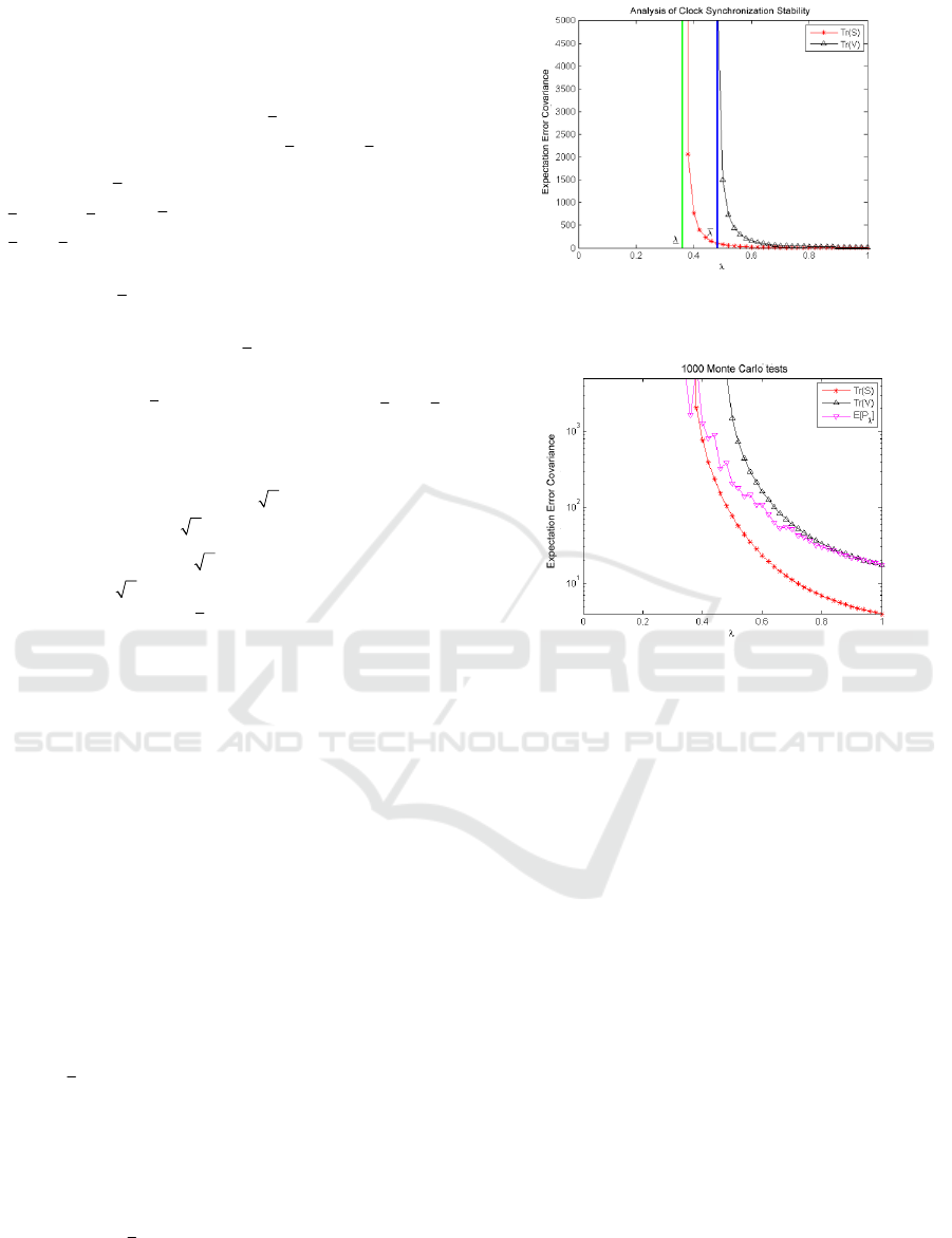
Figure.1. Upper and lower bounds transition from

unbounded to bounded

Figure.2. Monte Carlo test

The Monte Carlo simulation is used to simulate

the real clock synchronization process. The inverted

triangle curve in Figure. 2 represents the

synchronization error covariance

[]

, which is

obtained from 1000 Monte Carlo experiments. The

star of red curve and the black positive triangle curve

represents the lower bound and upper bound of the

steady-state error covariance, respectively, calculated

by the modified Riccati differential equation. In this

paper, when the actual arrival rate is 0,

lim [ ]

→∞

equal to infinity. It is obvious that the

synchronization error covariance based on Kalman

filter is a monotonically decreasing function of the

arrival rate. Note that when

0.36

, the

synchronization error covariance into the lower and

upper bound including area, when the measured

arrival rate is larger than the critical value, the

synchronization error covariance convergence, and

its convergence range in the lower and upper bound,

to prove the correctness of the theory.

The article propose a static state estimator for

linear systems:

γ ()

tttstt

Ax K y y

=+ −

)

))

(17)

Where,

represents the static gain constant.

ICECTT 2018 - 3rd International Conference on Electromechanical Control Technology and Transportation

226

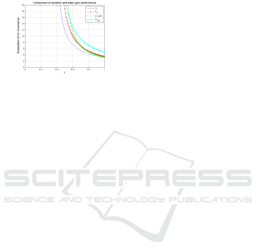
Figure.3. Comparison of dynamic and static gain

performance

Three static gain methods are proposed in the

reference (Sinopoli, 2004), and the Kalman filter

gain in this paper belongs to the dynamic gain. By

comparing the performance of these three kinds of

static gain, it is shown that the Kalman filter is still

the best when the measurement value is lost. Figure 3

compares the performance between the dynamic

Kalman filter gain and three kinds of static gain, the

star of red curve represents the average error

covariance of dynamic gain, with the actual

observation arrival rate increases, the most close to

the upper bound of convergence theory analysis. It is

shown that the steady-state error covariance is

minimum and the estimation algorithm is optimal.

6 CONCLUSIONS

This paper prove that there exists the critical arrival

rate of the measured value, and the average error

covariance changes from unboundedness to

boundedness with the arrival rate of the actual

measured value increasing and exceeding the critical

arrival rate. A numerical algorithm is proposed to

calculate the upper and lower bound of the critical

arrival rate and the boundary of the steady-state mean

error covariance. The simulation results show that the

average error covariance divergence and the clock

parameter estimation are unstable when the actual

measured value arrival rate is less than the

critical value. This theory can also guide the resource

allocation of wireless sensor networks. If the current

synchronization accuracy does not meet the

requirements, we can get better synchronization

accuracy by improving the communication resources.

REFERENCES

F Akyildiz, W.Su, Y.Sankaresubramaniam, and

E.Cayirci, 2002.Wireless sensor networks: a

survey[J]. Computer Networks, vol. 38, no. 4,

pp. 393-422.

Wu Y C, Chaudhari Q, Serpedin E.,2011. Clock

synchronization of wireless sensor netwoks[J].

IEEE Signal Processing Magazine, 28(1):

124-138.

Tao Zhi Yong, Ming Hu., 2012. Improvement Based

on the Hierarchical Levels Structure of the TPSN

Algorithm[J]. Chinese Journal of Sensors and

Actuators,5: 027.

Wakabayashi K, Isogai A, Watanabe D, et al., 2013.

Involvement of methionine salvage pathway

genes of Saccharomyces cerevisiae in the

production of precursor compounds of dimethyl

trisulfide (DMTS)[J]. Journal of bioscience and

bioengineering, 116(4): 475-479.

Wang T, Cai C Y, Guo D, et al., 2014. Clock

Synchronization in Wireless Sensor Networks: A

New Model and Analysis Approach Based on

Networked Control Perspective[J]. Mathematical

Problems in Engineering,(2014-8-31), 2014,

2014(3):1-19.

M. Micheli, 2001. Random Sampling of a

Continuous-time Stochastic Dynamical System:

Analysis, State Estimation, Applications,

Master’sThesis, University of California,

Berkeley.

M. Micheli and M. I. Jordan, 2002. Random

Sampling of a continuoustime stochastic

dynamical system, Proc. 15th Intl. Symposium on

the Mathematical Theory of Networks and

Systems (MTNS).

Wang T, Guo D, Cai C Y, et al., 2015. Clock

Synchronization in Wireless Sensor Networks:

Analysis and Design of Error Precision Based on

Lossy Networked Control Perspective [J].

Mathematical Problems in Engineering,

2015,(2015-4-8), 2015(2):1-17.

M.Alexiadis, P. Dokopoulos, and H. Sahsamanoglou,

1999. “Wind speedand power forecasting based

on spatial correlation models” IEEETrans.

Energy Convers., vol. 14, no. 3, pp. 836–842.

N N.M. Moayedi, Y. Foo, and Y. Soh, 2010. Adaptive

Kalman filtering in networked systems with

random sensor delays, multiple packet dropouts

and missing measurements[J]. IEEE Trans.

Signal Process., vol. 58, no.3, pp. 1577–1588.

Sinopoli B, Schenato L, Franceschetti M, et al., 2004.

Kalman filtering with intermittent observations

[J]. IEEE Transactions on Automatic Control,

1(9):1453-1464.

Stability Analysis of Clock Synchronization Algorithm over Lossy WSNs

227